DecisionBoundaryDisplay#
- class sklearn.inspection.DecisionBoundaryDisplay(*, xx0, xx1, n_classes, response, target_colors=None, xlabel=None, ylabel=None, multiclass_colors='deprecated')[source]#
Decisions boundary visualization.
It is recommended to use
from_estimatorto create aDecisionBoundaryDisplay. All parameters are stored as attributes.Read more in the User Guide.
For a detailed example comparing the decision boundaries of multinomial and one-vs-rest logistic regression, please see Decision Boundaries of Multinomial and One-vs-Rest Logistic Regression.
Added in version 1.1.
- Parameters:
- xx0ndarray of shape (grid_resolution, grid_resolution)
First output of
meshgrid.- xx1ndarray of shape (grid_resolution, grid_resolution)
Second output of
meshgrid.- n_classesint
Expected number of unique classes or labels if
responsewas generated by a classifier or a clusterer.For outlier detectors,
n_classesshould be set to 2 by definition (inlier or outlier).For regressors,
n_classesshould also be set to 2 by convention (continuous responses are displayed the same way as unthresholded binary responses).Added in version 1.9.
- responsendarray of shape (grid_resolution, grid_resolution) or (grid_resolution, grid_resolution, n_classes)
Values of the response function.
- target_colorsstr or list of matplotlib colors, default=None
Specifies how to color each class when plotting all classes of multiclass problems.
Possible inputs are:
None: defaults to list of accessible Petroff colors if
n_classes <= 10, otherwise ‘gist_rainbow’ colormapstr: name of
matplotlib.colors.Colormaplist: list of length
n_classesof matplotlib colors
Single color (fading to white) colormaps will be generated from the colors in the list or colors taken from the colormap, and passed to the
cmapparameter of theplot_method.When
response_method='predict'andplot_method='contour',target_colorsis ignored and the class boundaries are plotted in black instead as the boundary lines may overlap and the colors don’t necessarily correspond to the classes.For binary problems,
target_colorsis also ignored andcmaporcolorscan be passed as kwargs instead, otherwise, the default colormap (‘viridis’) is used.Added in version 1.10:
multiclass_colorswas renamed totarget_colors- xlabelstr, default=None
Default label to place on x axis.
- ylabelstr, default=None
Default label to place on y axis.
- multiclass_colorsstr or list of matplotlib colors, default=None
Specifies how to color each class when plotting all classes of multiclass problems.
Possible inputs are:
None: defaults to list of accessible Petroff colors if
n_classes <= 10, otherwise ‘gist_rainbow’ colormapstr: name of
matplotlib.colors.Colormaplist: list of length
n_classesof matplotlib colors
Single color (fading to white) colormaps will be generated from the colors in the list or colors taken from the colormap, and passed to the
cmapparameter of theplot_method.When
response_method='predict'andplot_method='contour',target_colorsis ignored and the class boundaries are plotted in black instead as the boundary lines may overlap and the colors don’t necessarily correspond to the classes.For binary problems,
target_colorsis also ignored andcmaporcolorscan be passed as kwargs instead, otherwise, the default colormap (‘viridis’) is used.Added in version 1.7.
Changed in version 1.9:
target_colorsis now also used whenresponse_method="predict", except for whenplot_method='contour', where it is ignored and “black” is used instead. The default colors changed from ‘tab10’ to the more accessible Petroff colors.Deprecated since version 1.10:
multiclass_colorswas renamed totarget_colorsin 1.10 and will be removed in 1.12.
- Attributes:
- surface_matplotlib
QuadContourSetorQuadMeshor list of such objects If
plot_methodis ‘contour’ or ‘contourf’,surface_isQuadContourSet. Ifplot_methodis ‘pcolormesh’,surface_isQuadMesh.- target_colors_array of shape (n_classes, 4)
Colors used to plot each class in multiclass problems. Only defined when
n_classes> 2.Added in version 1.10:
multiclass_colors_was renamed totarget_colors_- ax_matplotlib Axes
Axes with decision boundary.
- figure_matplotlib Figure
Figure containing the decision boundary.
- multiclass_colors_array of shape (n_classes, 4)
Colors used to plot each class in multiclass problems. Only defined when
n_classes> 2.Added in version 1.7.
Deprecated since version 1.10:
multiclass_colors_was renamed totarget_colors_in 1.10 and will be removed in 1.12.
- surface_matplotlib
See also
DecisionBoundaryDisplay.from_estimatorPlot decision boundary given an estimator.
Examples
>>> import matplotlib.pyplot as plt
>>> import matplotlib as mpl
>>> import numpy as np
>>> from sklearn.linear_model import LogisticRegression
>>> from sklearn.inspection import DecisionBoundaryDisplay
>>> data = np.array([[0, 0], [1, 1], [2, 1], [2, 2], [3, 2], [3, 3]])
>>> target = np.arange(data.shape[0])
>>> clf = LogisticRegression().fit(data, target)
>>> plot_methods = ["contourf", "contour", "pcolormesh"]
>>> response_methods = ["predict_proba", "decision_function", "predict"]
>>> _, axes = plt.subplots(
...     nrows=3,
...     ncols=3,
...     figsize=(12, 12),
...     constrained_layout=True
... )
>>> for plot_method_idx, plot_method in enumerate(plot_methods):
...     for response_method_idx, response_method in enumerate(response_methods):
...         ax = axes[plot_method_idx, response_method_idx]
...         display = DecisionBoundaryDisplay.from_estimator(
...             clf,
...             data,
...             grid_resolution=300,
...             response_method=response_method,
...             plot_method=plot_method,
...             ax=ax,
...             alpha=0.5,
...         )
...         cmap = mpl.colors.ListedColormap(display.target_colors_)
...         ax.scatter(
...             data[:, 0],
...             data[:, 1],
...             c=target.astype(int),
...             edgecolors="black",
...             cmap=cmap,
...         )
...         ax.set_title(
...             f"plot_method={plot_method}\nresponse_method={response_method}"
...         )
>>> plt.show()
- classmethod from_estimator(estimator, X, *, grid_resolution=100, eps=1.0, plot_method='contourf', response_method='auto', class_of_interest=None, target_colors=None, xlabel=None, ylabel=None, ax=None, multiclass_colors='deprecated', **kwargs)[source]#
Plot decision boundary given an estimator.
Read more in the User Guide.
- Parameters:
- estimatorobject
Trained estimator used to plot the decision boundary.
- X{array-like, sparse matrix, dataframe} of shape (n_samples, 2)
Input data that should be only 2-dimensional.
- grid_resolutionint, default=100
Number of grid points to use for plotting decision boundary. Higher values will make the plot look nicer but be slower to render.
- epsfloat, default=1.0
Extends the minimum and maximum values of X for evaluating the response function.
- plot_method{‘contourf’, ‘contour’, ‘pcolormesh’}, default=’contourf’
Plotting method to call when plotting the response. Please refer to the following matplotlib documentation for details:
contourf,contour,pcolormesh.- response_method{‘auto’, ‘decision_function’, ‘predict_proba’, ‘predict’}, default=’auto’
Specifies whether to use decision_function, predict_proba or predict as the target response. If set to ‘auto’, the response method is tried in the order as listed above.
Changed in version 1.6: For multiclass problems, ‘auto’ no longer defaults to ‘predict’.
- class_of_interestint, float, bool or str, default=None
The class to be plotted. For binary classifiers, if None,
estimator.classes_[1]is considered the positive class. For multiclass classifiers, if None, all classes will be represented in the decision boundary plot; whenresponse_methodis predict_proba or decision_function, the class with the highest response value at each point is plotted. The color of each class can be set viatarget_colors.Added in version 1.4.
- target_colorsstr or list of matplotlib colors, default=None
Specifies how to color each class when plotting multiclass problems and
class_of_interestis None.Possible inputs are:
None: defaults to list of accessible Petroff colors if
n_classes <= 10, otherwise ‘gist_rainbow’ colormapstr: name of
matplotlib.colors.Colormaplist: list of length
n_classesof matplotlib colors
Single color (fading to white) colormaps will be generated from the colors in the list or colors taken from the colormap, and passed to the
cmapparameter of theplot_method.When
response_method='predict'andplot_method='contour',target_colorsis ignored and the class boundaries are plotted in black instead as the boundary lines may overlap and the colors don’t necessarily correspond to the classes.For binary problems,
target_colorsis also ignored andcmaporcolorscan be passed as kwargs instead, otherwise, the default colormap (‘viridis’) is used.Added in version 1.10:
multiclass_colorswas renamed totarget_colors- xlabelstr, default=None
The label used for the x-axis. If
None, an attempt is made to extract a label fromXif it is a dataframe, otherwise an empty string is used.- ylabelstr, default=None
The label used for the y-axis. If
None, an attempt is made to extract a label fromXif it is a dataframe, otherwise an empty string is used.- axMatplotlib axes, default=None
Axes object to plot on. If
None, a new figure and axes is created.- multiclass_colorsstr or list of matplotlib colors, default=None
Specifies how to color each class when plotting all classes of multiclass problems.
Possible inputs are:
None: defaults to list of accessible Petroff colors if
n_classes <= 10, otherwise ‘gist_rainbow’ colormapstr: name of
matplotlib.colors.Colormaplist: list of length
n_classesof matplotlib colors
Single color (fading to white) colormaps will be generated from the colors in the list or colors taken from the colormap, and passed to the
cmapparameter of theplot_method.When
response_method='predict'andplot_method='contour',target_colorsis ignored and the class boundaries are plotted in black instead as the boundary lines may overlap and the colors don’t necessarily correspond to the classes.For binary problems,
target_colorsis also ignored andcmaporcolorscan be passed as kwargs instead, otherwise, the default colormap (‘viridis’) is used.Added in version 1.7.
Changed in version 1.9:
target_colorsis now also used whenresponse_method="predict", except for whenplot_method='contour', where it is ignored and “black” is used instead. The default colors changed from ‘tab10’ to the more accessible Petroff colors.Deprecated since version 1.10:
multiclass_colorswas renamed totarget_colorsin 1.10 and will be removed in 1.12.- **kwargsdict
Additional keyword arguments to be passed to the
plot_method.
- Returns:
- display
DecisionBoundaryDisplay Object that stores the result.
- display
See also
DecisionBoundaryDisplayDecision boundary visualization.
sklearn.metrics.ConfusionMatrixDisplay.from_estimatorPlot the confusion matrix given an estimator, the data, and the label.
sklearn.metrics.ConfusionMatrixDisplay.from_predictionsPlot the confusion matrix given the true and predicted labels.
Examples
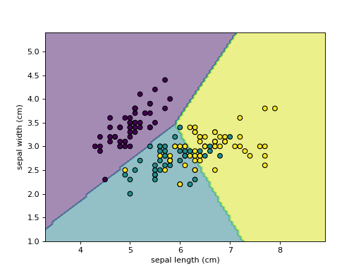
>>> import matplotlib as mpl
>>> import matplotlib.pyplot as plt
>>> from sklearn.datasets import load_iris
>>> from sklearn.linear_model import LogisticRegression
>>> from sklearn.inspection import DecisionBoundaryDisplay
>>> iris = load_iris()
>>> X = iris.data[:, :2]
>>> classifier = LogisticRegression().fit(X, iris.target)
>>> disp = DecisionBoundaryDisplay.from_estimator(
...     classifier, X, response_method="predict",
...     xlabel=iris.feature_names[0], ylabel=iris.feature_names[1],
...     alpha=0.5,
... )
>>> cmap = mpl.colors.ListedColormap(disp.target_colors_)
>>> disp.ax_.scatter(X[:, 0], X[:, 1], c=iris.target, edgecolor="k", cmap=cmap)
<...>
>>> plt.show()
- plot(plot_method='contourf', ax=None, xlabel=None, ylabel=None, **kwargs)[source]#
Plot visualization.
- Parameters:
- plot_method{‘contourf’, ‘contour’, ‘pcolormesh’}, default=’contourf’
Plotting method to call when plotting the response. Please refer to the following matplotlib documentation for details:
contourf,contour,pcolormesh.- axMatplotlib axes, default=None
Axes object to plot on. If
None, a new figure and axes is created.- xlabelstr, default=None
Overwrite the x-axis label.
- ylabelstr, default=None
Overwrite the y-axis label.
- **kwargsdict
Additional keyword arguments to be passed to the
plot_method. For binary problems,cmaporcolorscan be set here to specify the colormap or colors, otherwise the default colormap (‘viridis’) is used. If not specified by the user,zorderis set to -1 to ensure that the decision boundary is plotted in the background (in case a scatter plot is added on top).
- Returns:
- display:
DecisionBoundaryDisplay Object that stores computed values.
- display:
See also
DecisionBoundaryDisplay.from_estimatorPlot decision boundary given an estimator.
Examples
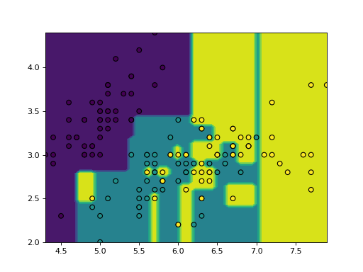
>>> import matplotlib as mpl
>>> import matplotlib.pyplot as plt
>>> import numpy as np
>>> from sklearn.datasets import load_iris
>>> from sklearn.inspection import DecisionBoundaryDisplay
>>> from sklearn.tree import DecisionTreeClassifier
>>> iris = load_iris()
>>> feature_1, feature_2 = np.meshgrid(
...     np.linspace(iris.data[:, 0].min(), iris.data[:, 0].max()),
...     np.linspace(iris.data[:, 1].min(), iris.data[:, 1].max())
... )
>>> grid = np.vstack([feature_1.ravel(), feature_2.ravel()]).T
>>> tree = DecisionTreeClassifier().fit(iris.data[:, :2], iris.target)
>>> y_pred = np.reshape(tree.predict(grid), feature_1.shape)
>>> display = DecisionBoundaryDisplay(
...     xx0=feature_1,
...     xx1=feature_2,
...     n_classes=len(tree.classes_),
...     response=y_pred
... )
>>> display.plot()
<...>
>>> display.ax_.scatter(
...     iris.data[:, 0],
...     iris.data[:, 1],
...     c=iris.target,
...     cmap=mpl.colors.ListedColormap(display.target_colors_),
...     edgecolor="black"
... )
<...>
>>> plt.show()
Gallery examples#
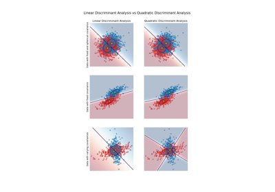
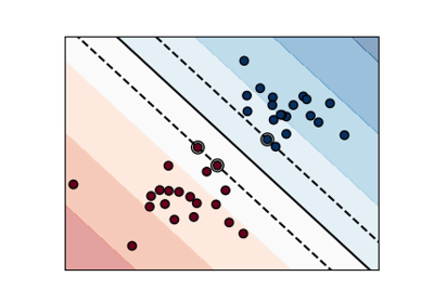
Linear and Quadratic Discriminant Analysis with covariance ellipsoid
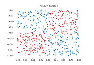
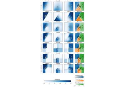
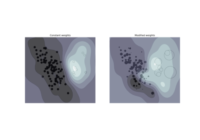
Visualizing the probabilistic predictions of a VotingClassifier
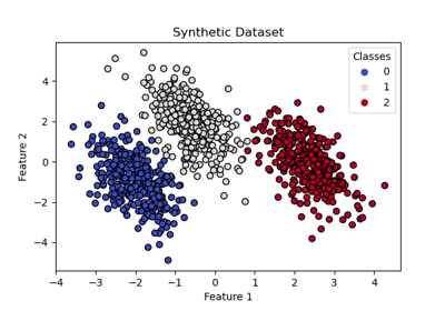
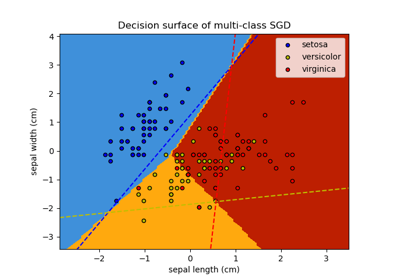
Decision Boundaries of Multinomial and One-vs-Rest Logistic Regression
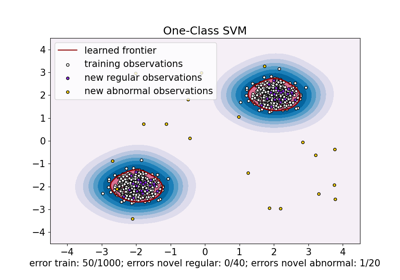
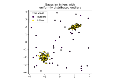
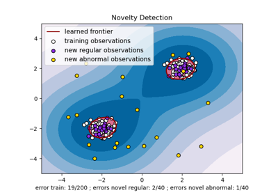
One-Class SVM versus One-Class SVM using Stochastic Gradient Descent
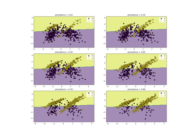
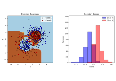
Class Likelihood Ratios to measure classification performance
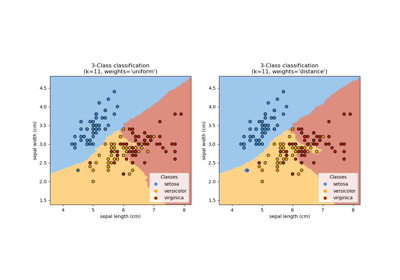
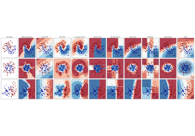
Comparing Nearest Neighbors with and without Neighborhood Components Analysis
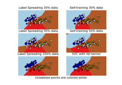
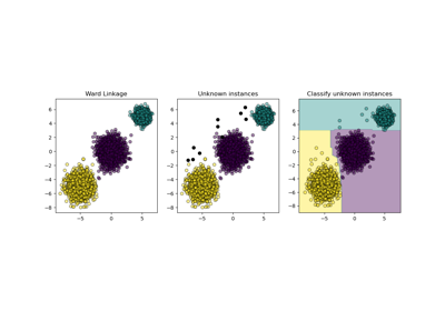
Decision boundary of semi-supervised classifiers versus SVM on the Iris dataset
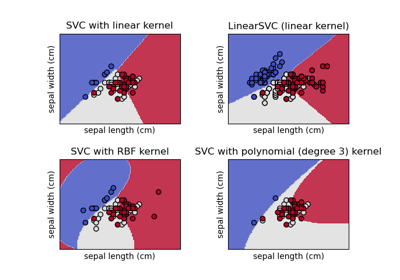
Plot different SVM classifiers in the iris dataset
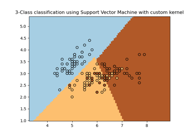
Plot classification boundaries with different SVM Kernels
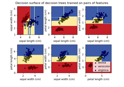
Plot the decision surface of decision trees trained on the iris dataset
