Note

Go to the end to download the full example code. or to run this example in your browser via JupyterLite or Binder

Linear and Quadratic Discriminant Analysis with covariance ellipsoid#

This example plots the covariance ellipsoids of each class and the decision boundary learned by LinearDiscriminantAnalysis (LDA) and QuadraticDiscriminantAnalysis (QDA). The ellipsoids display the double standard deviation for each class. With LDA, the standard deviation is the same for all the classes, while each class has its own standard deviation with QDA.

# Authors: The scikit-learn developers
# SPDX-License-Identifier: BSD-3-Clause

Data generation#

First, we define a function to generate synthetic data. It creates two blobs centered at (0, 0) and (1, 1). Each blob is assigned a specific class. The dispersion of the blob is controlled by the parameters cov_class_1 and cov_class_2, that are the covariance matrices used when generating the samples from the Gaussian distributions.

import numpy as np


def make_data(n_samples, n_features, cov_class_1, cov_class_2, seed=0):
    rng = np.random.RandomState(seed)
    X = np.concatenate(
        [
            rng.randn(n_samples, n_features) @ cov_class_1,
            rng.randn(n_samples, n_features) @ cov_class_2 + np.array([1, 1]),
        ]
    )
    y = np.concatenate([np.zeros(n_samples), np.ones(n_samples)])
    return X, y

We generate three datasets. In the first dataset, the two classes share the same covariance matrix, and this covariance matrix has the specificity of being spherical (isotropic). The second dataset is similar to the first one but does not enforce the covariance to be spherical. Finally, the third dataset has a non-spherical covariance matrix for each class.

covariance = np.array([[1, 0], [0, 1]])
X_isotropic_covariance, y_isotropic_covariance = make_data(
    n_samples=1_000,
    n_features=2,
    cov_class_1=covariance,
    cov_class_2=covariance,
    seed=0,
)
covariance = np.array([[0.0, -0.23], [0.83, 0.23]])
X_shared_covariance, y_shared_covariance = make_data(
    n_samples=300,
    n_features=2,
    cov_class_1=covariance,
    cov_class_2=covariance,
    seed=0,
)
cov_class_1 = np.array([[0.0, -1.0], [2.5, 0.7]]) * 2.0
cov_class_2 = cov_class_1.T
X_different_covariance, y_different_covariance = make_data(
    n_samples=300,
    n_features=2,
    cov_class_1=cov_class_1,
    cov_class_2=cov_class_2,
    seed=0,
)

Plotting Functions#

The code below is used to plot several pieces of information from the estimators used, i.e., LinearDiscriminantAnalysis (LDA) and QuadraticDiscriminantAnalysis (QDA). The displayed information includes:

the decision boundary based on the probability estimate of the estimator;
a scatter plot with circles representing the well-classified samples;
a scatter plot with crosses representing the misclassified samples;
the mean of each class, estimated by the estimator, marked with a star;
the estimated covariance represented by an ellipse at 2 standard deviations from the mean.

import matplotlib as mpl
from matplotlib import colors

from sklearn.inspection import DecisionBoundaryDisplay


def plot_ellipse(mean, cov, color, ax):
    v, w = np.linalg.eigh(cov)
    u = w[0] / np.linalg.norm(w[0])
    angle = np.arctan(u[1] / u[0])
    angle = 180 * angle / np.pi  # convert to degrees
    # filled Gaussian at 2 standard deviation
    ell = mpl.patches.Ellipse(
        mean,
        2 * v[0] ** 0.5,
        2 * v[1] ** 0.5,
        angle=180 + angle,
        facecolor=color,
        edgecolor="black",
        linewidth=2,
    )
    ell.set_clip_box(ax.bbox)
    ell.set_alpha(0.4)
    ax.add_artist(ell)


def plot_result(estimator, X, y, ax):
    cmap = colors.ListedColormap(["tab:red", "tab:blue"])
    DecisionBoundaryDisplay.from_estimator(
        estimator,
        X,
        response_method="predict_proba",
        plot_method="pcolormesh",
        ax=ax,
        cmap="RdBu",
        alpha=0.3,
    )
    DecisionBoundaryDisplay.from_estimator(
        estimator,
        X,
        response_method="predict_proba",
        plot_method="contour",
        ax=ax,
        alpha=1.0,
        levels=[0.5],
    )
    y_pred = estimator.predict(X)
    X_right, y_right = X[y == y_pred], y[y == y_pred]
    X_wrong, y_wrong = X[y != y_pred], y[y != y_pred]
    ax.scatter(X_right[:, 0], X_right[:, 1], c=y_right, s=20, cmap=cmap, alpha=0.5)
    ax.scatter(
        X_wrong[:, 0],
        X_wrong[:, 1],
        c=y_wrong,
        s=30,
        cmap=cmap,
        alpha=0.9,
        marker="x",
    )
    ax.scatter(
        estimator.means_[:, 0],
        estimator.means_[:, 1],
        c="yellow",
        s=200,
        marker="*",
        edgecolor="black",
    )

    if isinstance(estimator, LinearDiscriminantAnalysis):
        covariance = [estimator.covariance_] * 2
    else:
        covariance = estimator.covariance_
    plot_ellipse(estimator.means_[0], covariance[0], "tab:red", ax)
    plot_ellipse(estimator.means_[1], covariance[1], "tab:blue", ax)

    ax.set_box_aspect(1)
    ax.spines["top"].set_visible(False)
    ax.spines["bottom"].set_visible(False)
    ax.spines["left"].set_visible(False)
    ax.spines["right"].set_visible(False)
    ax.set(xticks=[], yticks=[])

Comparison of LDA and QDA#

We compare the two estimators LDA and QDA on all three datasets.

import matplotlib.pyplot as plt

from sklearn.discriminant_analysis import (
    LinearDiscriminantAnalysis,
    QuadraticDiscriminantAnalysis,
)

fig, axs = plt.subplots(nrows=3, ncols=2, sharex="row", sharey="row", figsize=(8, 12))

lda = LinearDiscriminantAnalysis(solver="svd", store_covariance=True)
qda = QuadraticDiscriminantAnalysis(store_covariance=True)

for ax_row, X, y in zip(
    axs,
    (X_isotropic_covariance, X_shared_covariance, X_different_covariance),
    (y_isotropic_covariance, y_shared_covariance, y_different_covariance),
):
    lda.fit(X, y)
    plot_result(lda, X, y, ax_row[0])
    qda.fit(X, y)
    plot_result(qda, X, y, ax_row[1])

axs[0, 0].set_title("Linear Discriminant Analysis")
axs[0, 0].set_ylabel("Data with fixed and spherical covariance")
axs[1, 0].set_ylabel("Data with fixed covariance")
axs[0, 1].set_title("Quadratic Discriminant Analysis")
axs[2, 0].set_ylabel("Data with varying covariances")
fig.suptitle(
    "Linear Discriminant Analysis vs Quadratic Discriminant Analysis",
    y=0.94,
    fontsize=15,
)
plt.show()

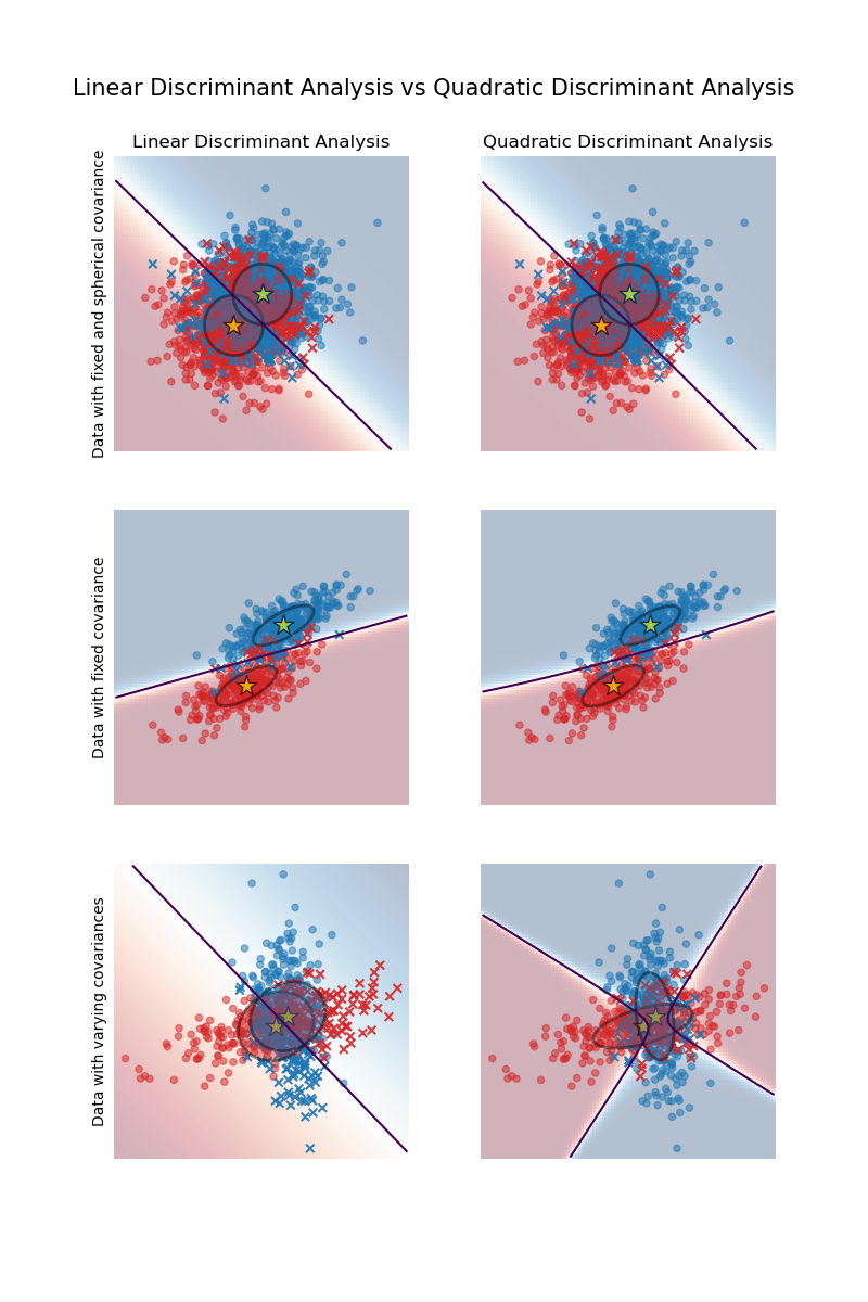
Linear Discriminant Analysis vs Quadratic Discriminant Analysis, Linear Discriminant Analysis, Quadratic Discriminant Analysis

The first important thing to notice is that LDA and QDA are equivalent for the first and second datasets. Indeed, the major difference is that LDA assumes that the covariance matrix of each class is equal, while QDA estimates a covariance matrix per class. Since in these cases the data generative process has the same covariance matrix for both classes, QDA estimates two covariance matrices that are (almost) equal and therefore equivalent to the covariance matrix estimated by LDA.

In the first dataset the covariance matrix used to generate the dataset is spherical, which results in a discriminant boundary that aligns with the perpendicular bisector between the two means. This is no longer the case for the second dataset. The discriminant boundary only passes through the middle of the two means.

Finally, in the third dataset, we observe the real difference between LDA and QDA. QDA fits two covariance matrices and provides a non-linear discriminant boundary, whereas LDA underfits since it assumes that both classes share a single covariance matrix.

Total running time of the script: (0 minutes 0.404 seconds)