Note

Go to the end to download the full example code. or to run this example in your browser via JupyterLite or Binder

Scalable learning with polynomial kernel approximation#

This example illustrates the use of PolynomialCountSketch to efficiently generate polynomial kernel feature-space approximations. This is used to train linear classifiers that approximate the accuracy of kernelized ones.

We use the Covtype dataset [2], trying to reproduce the experiments on the original paper of Tensor Sketch [1], i.e. the algorithm implemented by PolynomialCountSketch.

First, we compute the accuracy of a linear classifier on the original features. Then, we train linear classifiers on different numbers of features (n_components) generated by PolynomialCountSketch, approximating the accuracy of a kernelized classifier in a scalable manner.

# Authors: The scikit-learn developers
# SPDX-License-Identifier: BSD-3-Clause

Preparing the data#

Load the Covtype dataset, which contains 581,012 samples with 54 features each, distributed among 6 classes. The goal of this dataset is to predict forest cover type from cartographic variables only (no remotely sensed data). After loading, we transform it into a binary classification problem to match the version of the dataset in the LIBSVM webpage [2], which was the one used in [1].

from sklearn.datasets import fetch_covtype

X, y = fetch_covtype(return_X_y=True)

y[y != 2] = 0
y[y == 2] = 1  # We will try to separate class 2 from the other 6 classes.

Partitioning the data#

Here we select 5,000 samples for training and 10,000 for testing. To actually reproduce the results in the original Tensor Sketch paper, select 100,000 for training.

from sklearn.model_selection import train_test_split

X_train, X_test, y_train, y_test = train_test_split(
    X, y, train_size=5_000, test_size=10_000, random_state=42
)

Feature normalization#

Now scale features to the range [0, 1] to match the format of the dataset in the LIBSVM webpage, and then normalize to unit length as done in the original Tensor Sketch paper [1].

from sklearn.pipeline import make_pipeline
from sklearn.preprocessing import MinMaxScaler, Normalizer

mm = make_pipeline(MinMaxScaler(), Normalizer())
X_train = mm.fit_transform(X_train)
X_test = mm.transform(X_test)

Establishing a baseline model#

As a baseline, train a linear SVM on the original features and print the accuracy. We also measure and store accuracies and training times to plot them later.

import time

from sklearn.svm import LinearSVC

results = {}

lsvm = LinearSVC()
start = time.time()
lsvm.fit(X_train, y_train)
lsvm_time = time.time() - start
lsvm_score = 100 * lsvm.score(X_test, y_test)

results["LSVM"] = {"time": lsvm_time, "score": lsvm_score}
print(f"Linear SVM score on raw features: {lsvm_score:.2f}%")

Linear SVM score on raw features: 75.62%

Establishing the kernel approximation model#

Then we train linear SVMs on the features generated by PolynomialCountSketch with different values for n_components, showing that these kernel feature approximations improve the accuracy of linear classification. In typical application scenarios, n_components should be larger than the number of features in the input representation in order to achieve an improvement with respect to linear classification. As a rule of thumb, the optimum of evaluation score / run time cost is typically achieved at around n_components = 10 * n_features, though this might depend on the specific dataset being handled. Note that, since the original samples have 54 features, the explicit feature map of the polynomial kernel of degree four would have approximately 8.5 million features (precisely, 54^4). Thanks to PolynomialCountSketch, we can condense most of the discriminative information of that feature space into a much more compact representation. While we run the experiment only a single time (n_runs = 1) in this example, in practice one should repeat the experiment several times to compensate for the stochastic nature of PolynomialCountSketch.

from sklearn.kernel_approximation import PolynomialCountSketch

n_runs = 1
N_COMPONENTS = [250, 500, 1000, 2000]

for n_components in N_COMPONENTS:
    ps_lsvm_time = 0
    ps_lsvm_score = 0
    for _ in range(n_runs):
        pipeline = make_pipeline(
            PolynomialCountSketch(n_components=n_components, degree=4),
            LinearSVC(),
        )

        start = time.time()
        pipeline.fit(X_train, y_train)
        ps_lsvm_time += time.time() - start
        ps_lsvm_score += 100 * pipeline.score(X_test, y_test)

    ps_lsvm_time /= n_runs
    ps_lsvm_score /= n_runs

    results[f"LSVM + PS({n_components})"] = {
        "time": ps_lsvm_time,
        "score": ps_lsvm_score,
    }
    print(
        f"Linear SVM score on {n_components} PolynomialCountSketch "
        + f"features: {ps_lsvm_score:.2f}%"
    )

Linear SVM score on 250 PolynomialCountSketch features: 76.55%
Linear SVM score on 500 PolynomialCountSketch features: 76.92%
Linear SVM score on 1000 PolynomialCountSketch features: 77.79%
Linear SVM score on 2000 PolynomialCountSketch features: 78.59%

Establishing the kernelized SVM model#

Train a kernelized SVM to see how well PolynomialCountSketch is approximating the performance of the kernel. This, of course, may take some time, as the SVC class has a relatively poor scalability. This is the reason why kernel approximators are so useful:

from sklearn.svm import SVC

ksvm = SVC(C=500.0, kernel="poly", degree=4, coef0=0, gamma=1.0)

start = time.time()
ksvm.fit(X_train, y_train)
ksvm_time = time.time() - start
ksvm_score = 100 * ksvm.score(X_test, y_test)

results["KSVM"] = {"time": ksvm_time, "score": ksvm_score}
print(f"Kernel-SVM score on raw features: {ksvm_score:.2f}%")

Kernel-SVM score on raw features: 79.78%

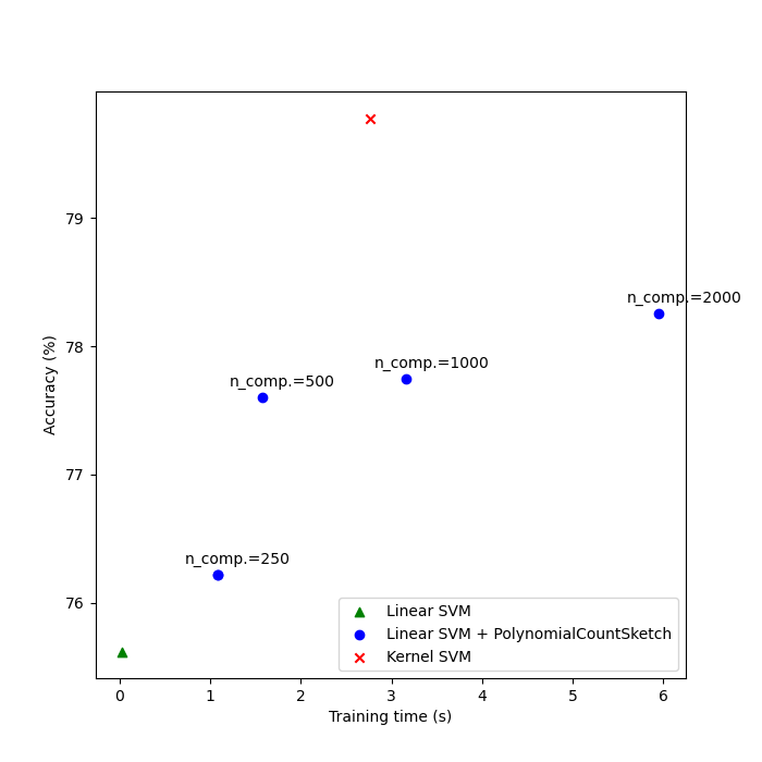
Comparing the results#

Finally, plot the results of the different methods against their training times. As we can see, the kernelized SVM achieves a higher accuracy, but its training time is much larger and, most importantly, will grow much faster if the number of training samples increases.

import matplotlib.pyplot as plt

fig, ax = plt.subplots(figsize=(7, 7))
ax.scatter(
    [
        results["LSVM"]["time"],
    ],
    [
        results["LSVM"]["score"],
    ],
    label="Linear SVM",
    c="green",
    marker="^",
)

ax.scatter(
    [
        results["LSVM + PS(250)"]["time"],
    ],
    [
        results["LSVM + PS(250)"]["score"],
    ],
    label="Linear SVM + PolynomialCountSketch",
    c="blue",
)

for n_components in N_COMPONENTS:
    ax.scatter(
        [
            results[f"LSVM + PS({n_components})"]["time"],
        ],
        [
            results[f"LSVM + PS({n_components})"]["score"],
        ],
        c="blue",
    )
    ax.annotate(
        f"n_comp.={n_components}",
        (
            results[f"LSVM + PS({n_components})"]["time"],
            results[f"LSVM + PS({n_components})"]["score"],
        ),
        xytext=(-30, 10),
        textcoords="offset pixels",
    )

ax.scatter(
    [
        results["KSVM"]["time"],
    ],
    [
        results["KSVM"]["score"],
    ],
    label="Kernel SVM",
    c="red",
    marker="x",
)

ax.set_xlabel("Training time (s)")
ax.set_ylabel("Accuracy (%)")
ax.legend()
plt.show()

References#

[1] Pham, Ninh and Rasmus Pagh. “Fast and scalable polynomial kernels via explicit feature maps.” KDD ‘13 (2013). https://doi.org/10.1145/2487575.2487591

[2] LIBSVM binary datasets repository https://www.csie.ntu.edu.tw/~cjlin/libsvmtools/datasets/binary.html

Total running time of the script: (0 minutes 21.081 seconds)