Features in Histogram Gradient Boosting Trees

Histogram-Based Gradient Boosting (HGBT) models may be one of the most useful supervised learning models in scikit-learn. They are based on a modern gradient boosting implementation comparable to LightGBM and XGBoost. As such, HGBT models are more feature rich than and often outperform alternative models like random forests, especially when the number of samples is larger than some ten thousands (see Comparing Random Forests and Histogram Gradient Boosting models).

The top usability features of HGBT models are:

1. Several available loss functions for mean and quantile regression tasks, see Quantile loss.

2. Categorical Features Support, see Categorical Feature Support in Gradient Boosting.

3. Early stopping.

4. Missing values support, which avoids the need for an imputer.

5. Monotonic Constraints.

6. Interaction constraints.

This example aims at showcasing all points except 2 and 6 in a real life setting.

# Author: Arturo Amor <david-arturo.amor-quiroz@inria.fr>
# License: BSD 3 clause

Preparing the data

The electricity dataset consists of data collected from the Australian New South Wales Electricity Market. In this market, prices are not fixed and are affected by supply and demand. They are set every five minutes. Electricity transfers to/from the neighboring state of Victoria were done to alleviate fluctuations.

The dataset, originally named ELEC2, contains 45,312 instances dated from 7 May 1996 to 5 December 1998. Each sample of the dataset refers to a period of 30 minutes, i.e. there are 48 instances for each time period of one day. Each sample on the dataset has 7 columns:

• date: between 7 May 1996 to 5 December 1998. Normalized between 0 and 1;

• day: day of week (1-7);

• period: half hour intervals over 24 hours. Normalized between 0 and 1;

• nswprice/nswdemand: electricity price/demand of New South Wales;

• vicprice/vicdemand: electricity price/demand of Victoria.

Originally, it is a classification task, but here we use it for the regression task to predict the scheduled electricity transfer between states.

from sklearn.datasets import fetch_openml

electricity = fetch_openml(
    name="electricity", version=1, as_frame=True, parser="pandas"
)
df = electricity.frame

This particular dataset has a stepwise constant target for the first 17,760 samples:

df["transfer"][:17_760].unique()

array([0.414912, 0.500526])

Let us drop those entries and explore the hourly electricity transfer over different days of the week:

import matplotlib.pyplot as plt
import seaborn as sns

df = electricity.frame.iloc[17_760:]
X = df.drop(columns=["transfer", "class"])
y = df["transfer"]

fig, ax = plt.subplots(figsize=(15, 10))
pointplot = sns.lineplot(x=df["period"], y=df["transfer"], hue=df["day"], ax=ax)
handles, lables = ax.get_legend_handles_labels()
ax.set(
    title="Hourly energy transfer for different days of the week",
    xlabel="Normalized time of the day",
    ylabel="Normalized energy transfer",
)
_ = ax.legend(handles, ["Sun", "Mon", "Tue", "Wed", "Thu", "Fri", "Sat"])

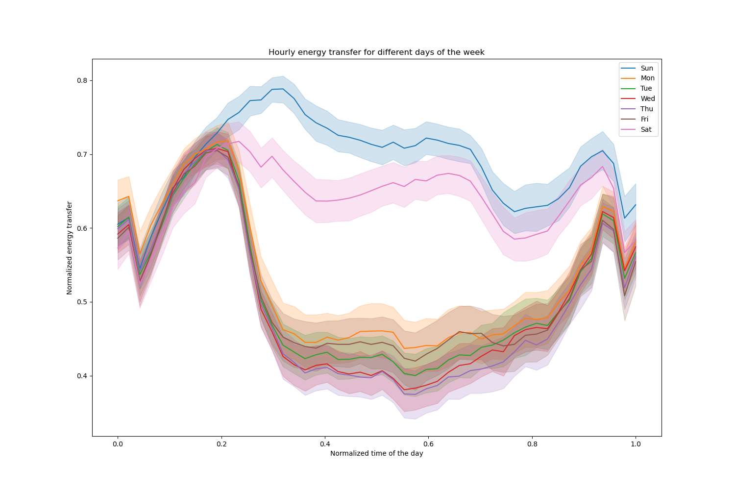
Notice that energy transfer increases systematically during weekends.

Effect of number of trees and early stopping

For the sake of illustrating the effect of the (maximum) number of trees, we train a HistGradientBoostingRegressor over the daily electricity transfer using the whole dataset. Then we visualize its predictions depending on the max_iter parameter. Here we don’t try to evaluate the performance of the model and its capacity to generalize but rather its capability to learn from the training data.

from sklearn.ensemble import HistGradientBoostingRegressor
from sklearn.model_selection import train_test_split

X_train, X_test, y_train, y_test = train_test_split(X, y, test_size=0.4, shuffle=False)

print(f"Training sample size: {X_train.shape[0]}")
print(f"Test sample size: {X_test.shape[0]}")
print(f"Number of features: {X_train.shape[1]}")

Training sample size: 16531
Test sample size: 11021
Number of features: 7

max_iter_list = [5, 50]
average_week_demand = (
    df.loc[X_test.index].groupby(["day", "period"], observed=False)["transfer"].mean()
)
colors = sns.color_palette("colorblind")
fig, ax = plt.subplots(figsize=(10, 5))
average_week_demand.plot(color=colors[0], label="recorded average", linewidth=2, ax=ax)

for idx, max_iter in enumerate(max_iter_list):
    hgbt = HistGradientBoostingRegressor(
        max_iter=max_iter, categorical_features=None, random_state=42
    )
    hgbt.fit(X_train, y_train)

    y_pred = hgbt.predict(X_test)
    prediction_df = df.loc[X_test.index].copy()
    prediction_df["y_pred"] = y_pred
    average_pred = prediction_df.groupby(["day", "period"], observed=False)[
        "y_pred"
    ].mean()
    average_pred.plot(
        color=colors[idx + 1], label=f"max_iter={max_iter}", linewidth=2, ax=ax
    )

ax.set(
    title="Predicted average energy transfer during the week",
    xticks=[(i + 0.2) * 48 for i in range(7)],
    xticklabels=["Sun", "Mon", "Tue", "Wed", "Thu", "Fri", "Sat"],
    xlabel="Time of the week",
    ylabel="Normalized energy transfer",
)
_ = ax.legend()

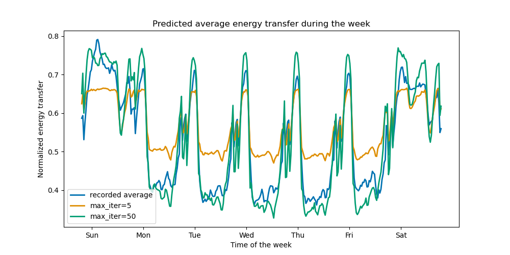
With just a few iterations, HGBT models can achieve convergence (see Comparing Random Forests and Histogram Gradient Boosting models), meaning that adding more trees does not improve the model anymore. In the figure above, 5 iterations are not enough to get good predictions. With 50 iterations, we are already able to do a good job.

Setting max_iter too high might degrade the prediction quality and cost a lot of avoidable computing resources. Therefore, the HGBT implementation in scikit-learn provides an automatic early stopping strategy. With it, the model uses a fraction of the training data as internal validation set (validation_fraction) and stops training if the validation score does not improve (or degrades) after n_iter_no_change iterations up to a certain tolerance (tol).

Notice that there is a trade-off between learning_rate and max_iter: Generally, smaller learning rates are preferable but require more iterations to converge to the minimum loss, while larger learning rates converge faster (less iterations/trees needed) but at the cost of a larger minimum loss.

Because of this high correlation between the learning rate the number of iterations, a good practice is to tune the learning rate along with all (important) other hyperparameters, fit the HBGT on the training set with a large enough value for max_iter and determine the best max_iter via early stopping and some explicit validation_fraction.

common_params = {
    "max_iter": 1_000,
    "learning_rate": 0.3,
    "validation_fraction": 0.2,
    "random_state": 42,
    "categorical_features": None,
    "scoring": "neg_root_mean_squared_error",
}

hgbt = HistGradientBoostingRegressor(early_stopping=True, **common_params)
hgbt.fit(X_train, y_train)

_, ax = plt.subplots()
plt.plot(-hgbt.validation_score_)
_ = ax.set(
    xlabel="number of iterations",
    ylabel="root mean squared error",
    title=f"Loss of hgbt with early stopping (n_iter={hgbt.n_iter_})",
)

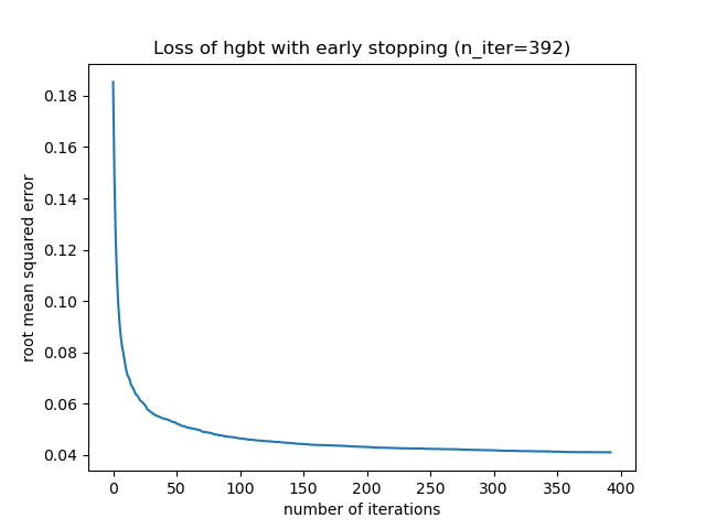
We can then overwrite the value for max_iter to a reasonable value and avoid the extra computational cost of the inner validation. Rounding up the number of iterations may account for variability of the training set:

import math

common_params["max_iter"] = math.ceil(hgbt.n_iter_ / 100) * 100
common_params["early_stopping"] = False
hgbt = HistGradientBoostingRegressor(**common_params)

Note

The inner validation done during early stopping is not optimal for time series.

Support for missing values

HGBT models have native support of missing values. During training, the tree grower decides where samples with missing values should go (left or right child) at each split, based on the potential gain. When predicting, these samples are sent to the learnt child accordingly. If a feature had no missing values during training, then for prediction, samples with missing values for that feature are sent to the child with the most samples (as seen during fit).

The present example shows how HGBT regressions deal with values missing completely at random (MCAR), i.e. the missingness does not depend on the observed data or the unobserved data. We can simulate such scenario by randomly replacing values from randomly selected features with nan values.

import numpy as np

from sklearn.metrics import root_mean_squared_error

rng = np.random.RandomState(42)
first_week = slice(0, 336)  # first week in the test set as 7 * 48 = 336
missing_fraction_list = [0, 0.01, 0.03]


def generate_missing_values(X, missing_fraction):
    total_cells = X.shape[0] * X.shape[1]
    num_missing_cells = int(total_cells * missing_fraction)
    row_indices = rng.choice(X.shape[0], num_missing_cells, replace=True)
    col_indices = rng.choice(X.shape[1], num_missing_cells, replace=True)
    X_missing = X.copy()
    X_missing.iloc[row_indices, col_indices] = np.nan
    return X_missing


fig, ax = plt.subplots(figsize=(12, 6))
ax.plot(y_test.values[first_week], label="Actual transfer")

for missing_fraction in missing_fraction_list:
    X_train_missing = generate_missing_values(X_train, missing_fraction)
    X_test_missing = generate_missing_values(X_test, missing_fraction)
    hgbt.fit(X_train_missing, y_train)
    y_pred = hgbt.predict(X_test_missing[first_week])
    rmse = root_mean_squared_error(y_test[first_week], y_pred)
    ax.plot(
        y_pred[first_week],
        label=f"missing_fraction={missing_fraction}, RMSE={rmse:.3f}",
        alpha=0.5,
    )
ax.set(
    title="Daily energy transfer predictions on data with MCAR values",
    xticks=[(i + 0.2) * 48 for i in range(7)],
    xticklabels=["Mon", "Tue", "Wed", "Thu", "Fri", "Sat", "Sun"],
    xlabel="Time of the week",
    ylabel="Normalized energy transfer",
)
_ = ax.legend(loc="lower right")

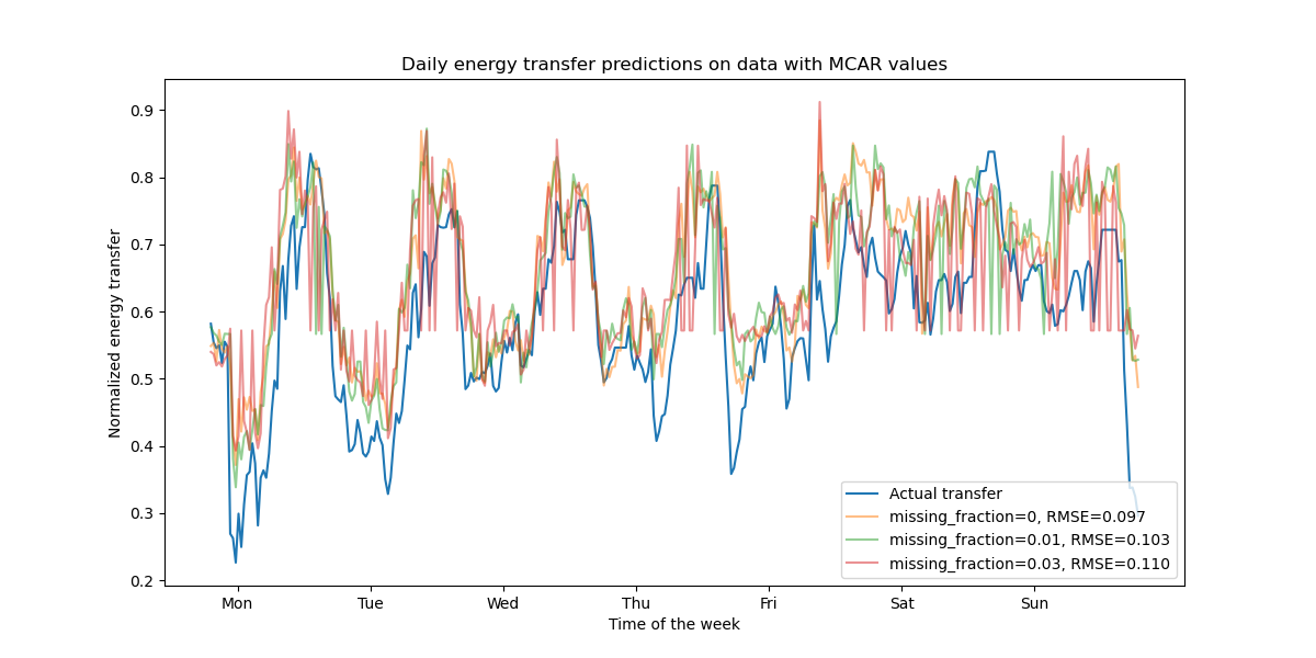
As expected, the model degrades as the proportion of missing values increases.

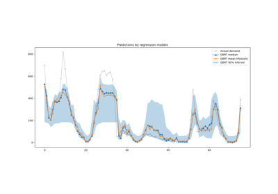
Support for quantile loss

The quantile loss in regression enables a view of the variability or uncertainty of the target variable. For instance, predicting the 5th and 95th percentiles can provide a 90% prediction interval, i.e. the range within which we expect a new observed value to fall with 90% probability.

from sklearn.metrics import mean_pinball_loss

quantiles = [0.95, 0.05]
predictions = []

fig, ax = plt.subplots(figsize=(12, 6))
ax.plot(y_test.values[first_week], label="Actual transfer")

for quantile in quantiles:
    hgbt_quantile = HistGradientBoostingRegressor(
        loss="quantile", quantile=quantile, **common_params
    )
    hgbt_quantile.fit(X_train, y_train)
    y_pred = hgbt_quantile.predict(X_test[first_week])

    predictions.append(y_pred)
    score = mean_pinball_loss(y_test[first_week], y_pred)
    ax.plot(
        y_pred[first_week],
        label=f"quantile={quantile}, pinball loss={score:.2f}",
        alpha=0.5,
    )

ax.fill_between(
    range(len(predictions[0][first_week])),
    predictions[0][first_week],
    predictions[1][first_week],
    color=colors[0],
    alpha=0.1,
)
ax.set(
    title="Daily energy transfer predictions with quantile loss",
    xticks=[(i + 0.2) * 48 for i in range(7)],
    xticklabels=["Mon", "Tue", "Wed", "Thu", "Fri", "Sat", "Sun"],
    xlabel="Time of the week",
    ylabel="Normalized energy transfer",
)
_ = ax.legend(loc="lower right")

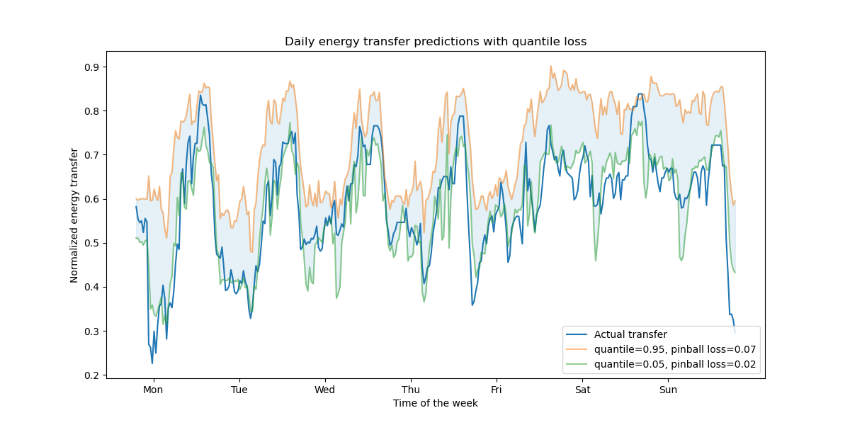
We observe a tendence to over-estimate the energy transfer. This could be be quantitatively confirmed by computing empirical coverage numbers as done in the calibration of confidence intervals section. Keep in mind that those predicted percentiles are just estimations from a model. One can still improve the quality of such estimations by:

• collecting more data-points;

• better tuning of the model hyperparameters, see Prediction Intervals for Gradient Boosting Regression;

• engineering more predictive features from the same data, see Time-related feature engineering.

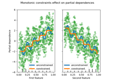
Monotonic constraints

Given specific domain knowledge that requires the relationship between a feature and the target to be monotonically increasing or decreasing, one can enforce such behaviour in the predictions of a HGBT model using monotonic constraints. This makes the model more interpretable and can reduce its variance (and potentially mitigate overfitting) at the risk of increasing bias. Monotonic constraints can also be used to enforce specific regulatory requirements, ensure compliance and align with ethical considerations.

In the present example, the policy of transferring energy from Victoria to New South Wales is meant to alleviate price fluctuations, meaning that the model predictions have to enforce such goal, i.e. transfer should increase with price and demand in New South Wales, but also decrease with price and demand in Victoria, in order to benefit both populations.

If the training data has feature names, it’s possible to specify the monotonic constraints by passing a dictionary with the convention:

• 1: monotonic increase

• 0: no constraint

• -1: monotonic decrease

Alternatively, one can pass an array-like object encoding the above convention by position.

from sklearn.inspection import PartialDependenceDisplay

monotonic_cst = {
    "date": 0,
    "day": 0,
    "period": 0,
    "nswdemand": 1,
    "nswprice": 1,
    "vicdemand": -1,
    "vicprice": -1,
}
hgbt_no_cst = HistGradientBoostingRegressor(
    categorical_features=None, random_state=42
).fit(X, y)
hgbt_cst = HistGradientBoostingRegressor(
    monotonic_cst=monotonic_cst, categorical_features=None, random_state=42
).fit(X, y)

fig, ax = plt.subplots(nrows=2, figsize=(15, 10))
disp = PartialDependenceDisplay.from_estimator(
    hgbt_no_cst,
    X,
    features=["nswdemand", "nswprice"],
    line_kw={"linewidth": 2, "label": "unconstrained", "color": "tab:blue"},
    ax=ax[0],
)
PartialDependenceDisplay.from_estimator(
    hgbt_cst,
    X,
    features=["nswdemand", "nswprice"],
    line_kw={"linewidth": 2, "label": "constrained", "color": "tab:orange"},
    ax=disp.axes_,
)
disp = PartialDependenceDisplay.from_estimator(
    hgbt_no_cst,
    X,
    features=["vicdemand", "vicprice"],
    line_kw={"linewidth": 2, "label": "unconstrained", "color": "tab:blue"},
    ax=ax[1],
)
PartialDependenceDisplay.from_estimator(
    hgbt_cst,
    X,
    features=["vicdemand", "vicprice"],
    line_kw={"linewidth": 2, "label": "constrained", "color": "tab:orange"},
    ax=disp.axes_,
)
_ = plt.legend()

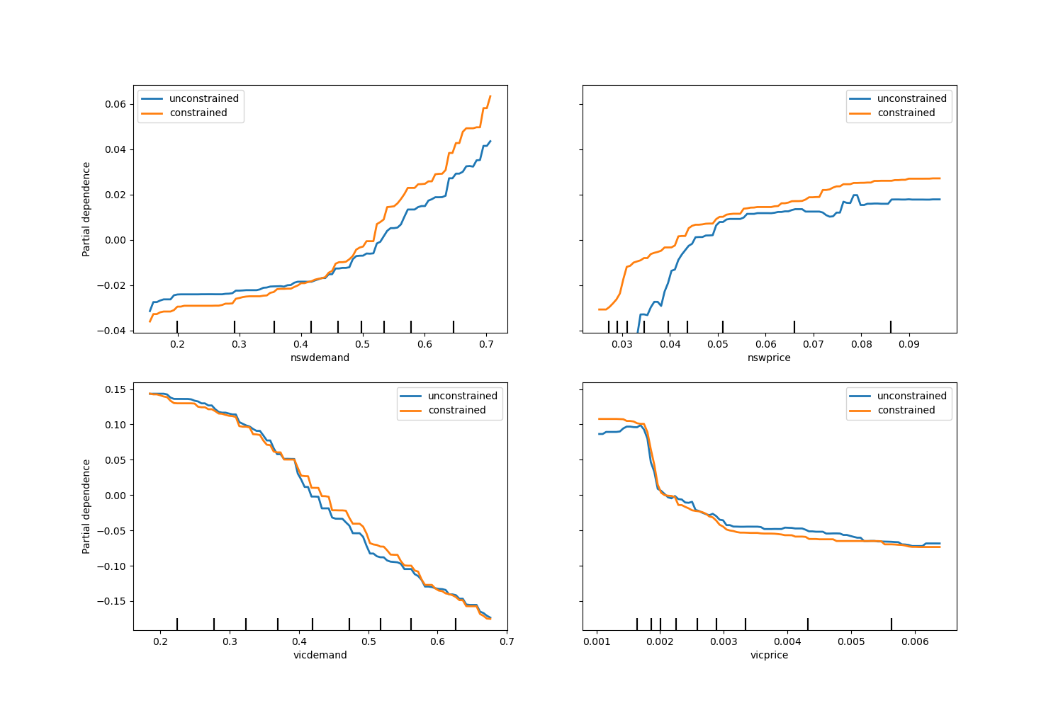
Observe that nswdemand and vicdemand seem already monotonic without constraint. This is a good example to show that the model with monotonicity constraints is “overconstraining”.

Additionally, we can verify that the predictive quality of the model is not significantly degraded by introducing the monotonic constraints. For such purpose we use TimeSeriesSplit cross-validation to estimate the variance of the test score. By doing so we guarantee that the training data does not succeed the testing data, which is crucial when dealing with data that have a temporal relationship.

from sklearn.metrics import make_scorer, root_mean_squared_error
from sklearn.model_selection import TimeSeriesSplit, cross_validate

ts_cv = TimeSeriesSplit(n_splits=5, gap=48, test_size=336)  # a week has 336 samples
scorer = make_scorer(root_mean_squared_error)

cv_results = cross_validate(hgbt_no_cst, X, y, cv=ts_cv, scoring=scorer)
rmse = cv_results["test_score"]
print(f"RMSE without constraints = {rmse.mean():.3f} +/- {rmse.std():.3f}")

cv_results = cross_validate(hgbt_cst, X, y, cv=ts_cv, scoring=scorer)
rmse = cv_results["test_score"]
print(f"RMSE with constraints    = {rmse.mean():.3f} +/- {rmse.std():.3f}")

RMSE without constraints = 0.103 +/- 0.030
RMSE with constraints    = 0.107 +/- 0.034

That being said, notice the comparison is between two different models that may be optimized by a different combination of hyperparameters. That is the reason why we do no use the common_params in this section as done before.

Related examples

Lagged features for time series forecasting

Lagged features for time series forecasting

Comparing Random Forests and Histogram Gradient Boosting models

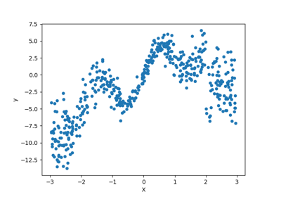
Comparing Random Forests and Histogram Gradient Boosting models

Monotonic Constraints

Monotonic Constraints

Time-related feature engineering

Time-related feature engineering

Release Highlights for scikit-learn 0.23

Release Highlights for scikit-learn 0.23