Note
Go to the end to download the full example code or to run this example in your browser via JupyterLite or Binder.
Compare BIRCH and MiniBatchKMeans#
This example compares the timing of BIRCH (with and without the global clustering step) and MiniBatchKMeans on a synthetic dataset having 25,000 samples and 2 features generated using make_blobs.
Both MiniBatchKMeans and BIRCH are very scalable algorithms and could
run efficiently on hundreds of thousands or even millions of datapoints. We
chose to limit the dataset size of this example in the interest of keeping
our Continuous Integration resource usage reasonable but the interested
reader might enjoy editing this script to rerun it with a larger value for
n_samples.
If n_clusters is set to None, the data is reduced from 25,000
samples to a set of 158 clusters. This can be viewed as a preprocessing
step before the final (global) clustering step that further reduces these
158 clusters to 100 clusters.
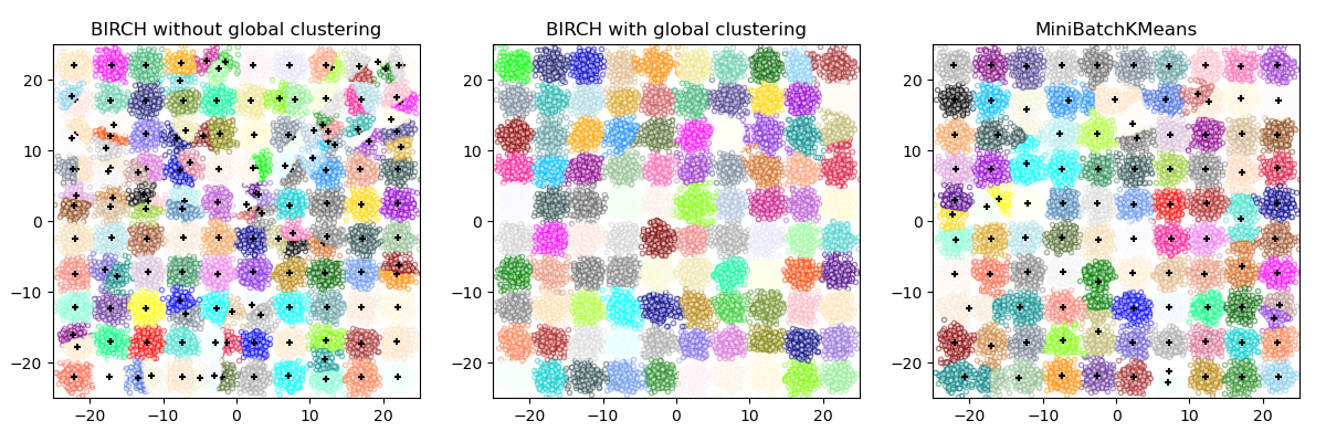
BIRCH without global clustering as the final step took 0.47 seconds
n_clusters : 158
BIRCH with global clustering as the final step took 0.48 seconds
n_clusters : 100
Time taken to run MiniBatchKMeans 0.22 seconds
# Authors: The scikit-learn developers
# SPDX-License-Identifier: BSD-3-Clause

from itertools import cycle
from time import time

import matplotlib.colors as colors
import matplotlib.pyplot as plt
import numpy as np
from joblib import cpu_count

from sklearn.cluster import Birch, MiniBatchKMeans
from sklearn.datasets import make_blobs

# Generate centers for the blobs so that it forms a 10 X 10 grid.
xx = np.linspace(-22, 22, 10)
yy = np.linspace(-22, 22, 10)
xx, yy = np.meshgrid(xx, yy)
n_centers = np.hstack((np.ravel(xx)[:, np.newaxis], np.ravel(yy)[:, np.newaxis]))

# Generate blobs to do a comparison between MiniBatchKMeans and BIRCH.
X, y = make_blobs(n_samples=25000, centers=n_centers, random_state=0)

# Use all colors that matplotlib provides by default.
colors_ = cycle(colors.cnames.keys())

fig = plt.figure(figsize=(12, 4))
fig.subplots_adjust(left=0.04, right=0.98, bottom=0.1, top=0.9)

# Compute clustering with BIRCH with and without the final clustering step
# and plot.
birch_models = [
    Birch(threshold=1.7, n_clusters=None),
    Birch(threshold=1.7, n_clusters=100),
]
final_step = ["without global clustering", "with global clustering"]

for ind, (birch_model, info) in enumerate(zip(birch_models, final_step)):
    t = time()
    birch_model.fit(X)
    print("BIRCH %s as the final step took %0.2f seconds" % (info, (time() - t)))

    # Plot result
    labels = birch_model.labels_
    centroids = birch_model.subcluster_centers_
    n_clusters = np.unique(labels).size
    print("n_clusters : %d" % n_clusters)

    ax = fig.add_subplot(1, 3, ind + 1)
    for this_centroid, k, col in zip(centroids, range(n_clusters), colors_):
        mask = labels == k
        ax.scatter(X[mask, 0], X[mask, 1], c="w", edgecolor=col, marker=".", alpha=0.5)
        if birch_model.n_clusters is None:
            ax.scatter(this_centroid[0], this_centroid[1], marker="+", c="k", s=25)
    ax.set_ylim([-25, 25])
    ax.set_xlim([-25, 25])
    ax.set_autoscaley_on(False)
    ax.set_title("BIRCH %s" % info)

# Compute clustering with MiniBatchKMeans.
mbk = MiniBatchKMeans(
    init="k-means++",
    n_clusters=100,
    batch_size=256 * cpu_count(),
    n_init=10,
    max_no_improvement=10,
    verbose=0,
    random_state=0,
)
t0 = time()
mbk.fit(X)
t_mini_batch = time() - t0
print("Time taken to run MiniBatchKMeans %0.2f seconds" % t_mini_batch)
mbk_means_labels_unique = np.unique(mbk.labels_)

ax = fig.add_subplot(1, 3, 3)
for this_centroid, k, col in zip(mbk.cluster_centers_, range(n_clusters), colors_):
    mask = mbk.labels_ == k
    ax.scatter(X[mask, 0], X[mask, 1], marker=".", c="w", edgecolor=col, alpha=0.5)
    ax.scatter(this_centroid[0], this_centroid[1], marker="+", c="k", s=25)
ax.set_xlim([-25, 25])
ax.set_ylim([-25, 25])
ax.set_title("MiniBatchKMeans")
ax.set_autoscaley_on(False)
plt.show()
Total running time of the script: (0 minutes 3.286 seconds)
Related examples
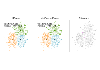
Comparison of the K-Means and MiniBatchKMeans clustering algorithms
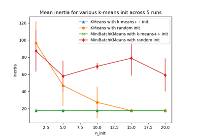
Empirical evaluation of the impact of k-means initialization
Comparing different clustering algorithms on toy datasets
