Note
Go to the end to download the full example code or to run this example in your browser via JupyterLite or Binder.
Multi-dimensional scaling#
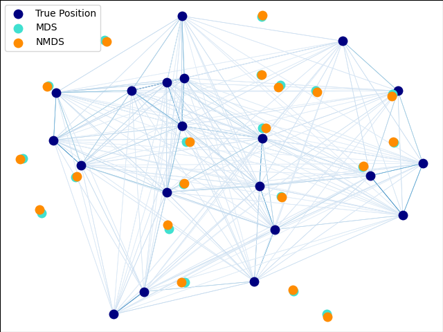
An illustration of the metric and non-metric MDS on generated noisy data.
# Authors: The scikit-learn developers
# SPDX-License-Identifier: BSD-3-Clause
Dataset preparation#
We start by uniformly generating 20 points in a 2D space.
import numpy as np
from matplotlib import pyplot as plt
from matplotlib.collections import LineCollection

from sklearn import manifold
from sklearn.decomposition import PCA
from sklearn.metrics import euclidean_distances

# Generate the data
EPSILON = np.finfo(np.float32).eps
n_samples = 20
rng = np.random.RandomState(seed=3)
X_true = rng.randint(0, 20, 2 * n_samples).astype(float)
X_true = X_true.reshape((n_samples, 2))

# Center the data
X_true -= X_true.mean()
Now we compute pairwise distances between all points and add a small amount of noise to the distance matrix. We make sure to keep the noisy distance matrix symmetric.
# Compute pairwise Euclidean distances
distances = euclidean_distances(X_true)

# Add noise to the distances
noise = rng.rand(n_samples, n_samples)
noise = noise + noise.T
np.fill_diagonal(noise, 0)
distances += noise
Here we compute metric, non-metric, and classical MDS of the noisy distance matrix.
mds = manifold.MDS(
    n_components=2,
    max_iter=3000,
    eps=1e-9,
    n_init=1,
    random_state=42,
    metric="precomputed",
    n_jobs=1,
    init="classical_mds",
)
X_mds = mds.fit(distances).embedding_

nmds = manifold.MDS(
    n_components=2,
    metric_mds=False,
    max_iter=3000,
    eps=1e-12,
    metric="precomputed",
    random_state=42,
    n_jobs=1,
    n_init=1,
    init="classical_mds",
)
X_nmds = nmds.fit_transform(distances)

cmds = manifold.ClassicalMDS(
    n_components=2,
    metric="precomputed",
)
X_cmds = cmds.fit_transform(distances)
Rescaling the non-metric MDS solution to match the spread of the original data.
To make the visual comparisons easier, we rotate the original data and all MDS solutions to their PCA axes. And flip horizontal and vertical MDS axes, if needed, to match the original data orientation.
# Rotate the data (CMDS does not need to be rotated, it is inherently PCA-aligned)
pca = PCA(n_components=2)
X_true = pca.fit_transform(X_true)
X_mds = pca.fit_transform(X_mds)
X_nmds = pca.fit_transform(X_nmds)

# Align the sign of PCs
for i in [0, 1]:
    if np.corrcoef(X_mds[:, i], X_true[:, i])[0, 1] < 0:
        X_mds[:, i] *= -1
    if np.corrcoef(X_nmds[:, i], X_true[:, i])[0, 1] < 0:
        X_nmds[:, i] *= -1
    if np.corrcoef(X_cmds[:, i], X_true[:, i])[0, 1] < 0:
        X_cmds[:, i] *= -1
Finally, we plot the original data and all MDS reconstructions.
fig = plt.figure(1)
ax = plt.axes([0.0, 0.0, 1.0, 1.0])

s = 100
plt.scatter(X_true[:, 0], X_true[:, 1], color="navy", s=s, lw=0, label="True Position")
plt.scatter(X_mds[:, 0], X_mds[:, 1], color="turquoise", s=s, lw=0, label="MDS")
plt.scatter(
    X_nmds[:, 0], X_nmds[:, 1], color="darkorange", s=s, lw=0, label="Non-metric MDS"
)
plt.scatter(
    X_cmds[:, 0], X_cmds[:, 1], color="lightcoral", s=s, lw=0, label="Classical MDS"
)
plt.legend(scatterpoints=1, loc="best", shadow=False)

# Plot the edges
start_idx, end_idx = X_mds.nonzero()
# a sequence of (*line0*, *line1*, *line2*), where::
#            linen = (x0, y0), (x1, y1), ... (xm, ym)
segments = [
    [X_true[i, :], X_true[j, :]] for i in range(len(X_true)) for j in range(len(X_true))
]
edges = distances.max() / (distances + EPSILON) * 100
np.fill_diagonal(edges, 0)
edges = np.abs(edges)
lc = LineCollection(
    segments, zorder=0, cmap=plt.cm.Blues, norm=plt.Normalize(0, edges.max())
)
lc.set_array(edges.flatten())
lc.set_linewidths(np.full(len(segments), 0.5))
ax.add_collection(lc)

plt.show()
Total running time of the script: (0 minutes 0.173 seconds)
Related examples
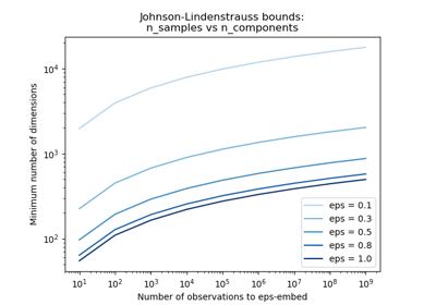
The Johnson-Lindenstrauss bound for embedding with random projections
