Comparing randomized search and grid search for hyperparameter estimation

Compare several strategies to optimize the hyperparameters of a linear SVM trained with stochastic gradient descent. We score the candidates with the one-vs-rest ROC AUC (roc_auc_ovr), which evaluates the ranking quality of the predicted class probabilities rather than the raw accuracy of the hard labels.

We start with an exhaustive grid search (GridSearchCV) that evaluates every combination of a discretized parameter grid. Because the grid is fixed, we are forced to fit every configuration and we may even miss a good combination that falls between two grid points.

We then run a randomized search (RandomizedSearchCV) that samples the parameter space instead of discretizing it. With a smaller budget it explores the space more efficiently and reaches an equivalent solution with fewer iterations.

Finally, we run a successive halving search (HalvingRandomSearchCV) that samples even more candidates but keeps the cost low by evaluating them on a small number of training samples first and discarding the unpromising ones early. It combines a large number of candidates with a reduced fit and predict time in the early iterations.

# Authors: The scikit-learn developers
# SPDX-License-Identifier: BSD-3-Clause

Loading the dataset

We use the digits dataset and restrict ourselves to the first three classes to keep the problem small and the search fast.

from sklearn.datasets import load_digits

X, y = load_digits(return_X_y=True, n_class=3)

Defining the estimator

We optimize a linear SVM trained with stochastic gradient descent (SGDClassifier). We use the "modified_huber" loss, a smoothed variant of the hinge loss: it keeps the large-margin behavior of a linear SVM while also exposing predict_proba. The probability estimates are required to score the candidates with the one-vs-rest ROC AUC, which the plain hinge loss could not provide.

from sklearn.linear_model import SGDClassifier

linear_svm = SGDClassifier(
    loss="modified_huber",
    penalty="elasticnet",
    fit_intercept=True,
    max_iter=5_000,
)

The report helper below prints the best parameter settings found by a given search so that we can compare the different strategies.

Successive halving stores in cv_results_ the candidates evaluated at every iteration, on increasing amounts of resources. The early iterations are scored on a small subset of the data, where perfect but unreliable scores are common. To keep the comparison fair, when an "iter" column is present we only keep the last iteration, i.e. the surviving candidates trained on the full set of resources, and we rank candidates by their mean validation score.

import pandas as pd


def report(results, n_top=3):
    """Report the top parameters for each search strategy."""
    results = pd.DataFrame(results)
    if "iter" in results:
        results = results[results["iter"] == results["iter"].max()]

    for rank, (_, candidate) in enumerate(
        results.nlargest(n_top, "mean_test_score").iterrows(), start=1
    ):
        print(
            f"Model with rank: {rank}\n"
            f"Mean validation score: "
            f"{candidate['mean_test_score']:.3f} "
            f"(std: {candidate['std_test_score']:.3f})\n"
            f"Parameters: {candidate['params']}\n"
        )

Grid search

GridSearchCV explores the entire parameter space defined as a grid. Continuous parameters therefore have to be discretized beforehand and every combination of the grid is evaluated. Two limitations follow from this design: we are forced to fit and score each configuration, even the unpromising ones, and the best hyperparameters may lie between two grid points and thus be missed entirely.

Some configurations do not let SGDClassifier converge and raise a ConvergenceWarning. These correspond to the poorly performing configurations that the search is meant to explore and discard, so it is fine to silence the warning with a warnings.catch_warnings context manager to keep the output readable.

import warnings
from time import time

import numpy as np

from sklearn.exceptions import ConvergenceWarning
from sklearn.model_selection import GridSearchCV

param_grid = {
    "average": [True, False],
    "l1_ratio": np.linspace(0, 1, num=10),
    "alpha": np.power(10, np.arange(-2, 1, dtype=float)),
}

grid_search = GridSearchCV(linear_svm, param_grid=param_grid, scoring="roc_auc_ovr")
start = time()
with warnings.catch_warnings():
    warnings.simplefilter("ignore", category=ConvergenceWarning)
    grid_search.fit(X, y)

print(
    f"GridSearchCV took {time() - start:.2f} seconds for "
    f"{len(grid_search.cv_results_['params'])} candidate parameter settings."
)
report(grid_search.cv_results_)

GridSearchCV took 137.46 seconds for 60 candidate parameter settings.
Model with rank: 1
Mean validation score: 1.000 (std: 0.000)
Parameters: {'alpha': np.float64(0.01), 'average': False, 'l1_ratio': np.float64(0.5555555555555556)}

Model with rank: 2
Mean validation score: 1.000 (std: 0.000)
Parameters: {'alpha': np.float64(0.1), 'average': False, 'l1_ratio': np.float64(0.0)}

Model with rank: 3
Mean validation score: 1.000 (std: 0.000)
Parameters: {'alpha': np.float64(1.0), 'average': False, 'l1_ratio': np.float64(0.0)}

Randomized search

RandomizedSearchCV samples a fixed number of candidates from the parameter distributions instead of evaluating a predefined grid. Sampling lets us explore the continuous distributions directly and spend our budget where it matters. Here we use only half as many candidates as the grid above, yet the randomized search reaches results equivalent to the grid search while fitting far fewer configurations.

import scipy.stats as stats

from sklearn.model_selection import RandomizedSearchCV

param_dist = {
    "average": [True, False],
    "l1_ratio": stats.uniform(0, 1),
    "alpha": stats.loguniform(1e-2, 1e0),
}

n_iter_search = 30
random_search = RandomizedSearchCV(
    linear_svm,
    param_distributions=param_dist,
    n_iter=n_iter_search,
    scoring="roc_auc_ovr",
    random_state=42,
)

start = time()
with warnings.catch_warnings():
    warnings.simplefilter("ignore", category=ConvergenceWarning)
    random_search.fit(X, y)
print(
    f"RandomizedSearchCV took {time() - start:.2f} seconds for {n_iter_search} "
    f"candidates parameter settings."
)
report(random_search.cv_results_)

RandomizedSearchCV took 55.49 seconds for 30 candidates parameter settings.
Model with rank: 1
Mean validation score: 1.000 (std: 0.000)
Parameters: {'alpha': np.float64(0.1673808578875213), 'average': False, 'l1_ratio': np.float64(0.04666566321361543)}

Model with rank: 2
Mean validation score: 1.000 (std: 0.000)
Parameters: {'alpha': np.float64(0.04649617447336333), 'average': False, 'l1_ratio': np.float64(0.7080725777960455)}

Model with rank: 3
Mean validation score: 1.000 (std: 0.000)
Parameters: {'alpha': np.float64(0.3503398491158687), 'average': False, 'l1_ratio': np.float64(0.2934881747180381)}

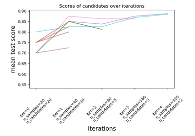
Successive halving search

HalvingRandomSearchCV samples candidates like the randomized search, but evaluates them on increasing amounts of resources (here the number of training samples). It starts with many candidates trained on a small subset of the data and, at each iteration, keeps only the most promising ones and grants them more samples. We therefore get the best of both worlds: a large number of candidates – which makes it more likely to find a good configuration – while keeping the fit and predict cost low in the early iterations where most candidates are discarded.

from sklearn.experimental import enable_halving_search_cv  # noqa: F401
from sklearn.model_selection import HalvingRandomSearchCV

n_candidates = 60
halving_search = HalvingRandomSearchCV(
    linear_svm,
    param_distributions=param_dist,
    n_candidates=n_candidates,
    scoring="roc_auc_ovr",
    random_state=42,
    min_resources=100,
)
start = time()
with warnings.catch_warnings():
    warnings.simplefilter("ignore", category=ConvergenceWarning)
    halving_search.fit(X, y)

print(
    f"HalvingRandomSearchCV took {time() - start:.2f} seconds for "
    f"{halving_search.n_candidates_[0]} initial candidate parameter settings."
)
report(halving_search.cv_results_)

HalvingRandomSearchCV took 56.90 seconds for 60 initial candidate parameter settings.
Model with rank: 1
Mean validation score: 1.000 (std: 0.000)
Parameters: {'alpha': np.float64(0.7121996518301618), 'average': False, 'l1_ratio': np.float64(0.11586905952512971)}

Model with rank: 2
Mean validation score: 1.000 (std: 0.001)
Parameters: {'alpha': np.float64(0.21137059440645725), 'average': False, 'l1_ratio': np.float64(0.4251558744912447)}

Model with rank: 3
Mean validation score: 0.999 (std: 0.001)
Parameters: {'alpha': np.float64(0.697828126512603), 'average': False, 'l1_ratio': np.float64(0.5704439744053994)}

Conclusion

Running the three searches on the same problem highlights their trade-offs:

• Grid search evaluates all 60 combinations of the grid and reaches a best mean validation ROC AUC of essentially 1.0. It is exhaustive, but its cost grows with the resolution of the grid and a finer grid would be needed to refine the continuous parameters, making it the slowest of the three.

• Randomized search reaches an essentially equivalent score while sampling only 30 candidates, i.e. half the budget, and is therefore markedly faster. Drawing the continuous parameters from distributions is usually a better use of a limited budget than refining a grid.

• Successive halving screens the 60 candidates for a run time comparable to the randomized search by spending most of its resources only on the most promising candidates. It explores more candidates than the randomized search without paying the full cost of the grid search.

A word of caution when reading the halving output: the cv_results_ of HalvingRandomSearchCV aggregates every iteration, including the first ones evaluated on very few samples where perfect but unreliable scores are common. This is why the report helper above keeps only the last iteration for the halving search, so that the reported scores are computed on the full set of resources and remain comparable to the grid and randomized searches. More generally, rely on best_params_ – which the halving search selects among the last-iteration candidates – and confirm the chosen model on a held-out test set.

Related examples

Successive Halving Iterations

Successive Halving Iterations

Analysis of the convergence of penalized logistic regression models

Analysis of the convergence of penalized logistic regression models

Custom refit strategy of a grid search with cross-validation

Custom refit strategy of a grid search with cross-validation

Comparison between grid search and successive halving

Comparison between grid search and successive halving