Note

Go to the end to download the full example code. or to run this example in your browser via JupyterLite or Binder

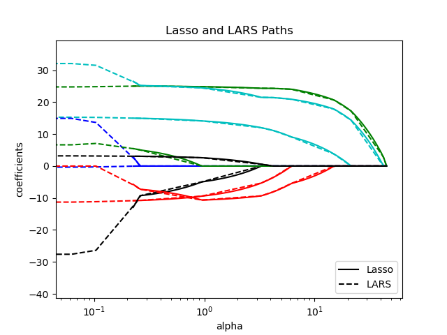
Lasso, Lasso-LARS, and Elastic Net paths#

This example shows how to compute the “paths” of coefficients along the Lasso, Lasso-LARS, and Elastic Net regularization paths. In other words, it shows the relationship between the regularization parameter (alpha) and the coefficients.

Lasso and Lasso-LARS impose a sparsity constraint on the coefficients, encouraging some of them to be zero. Elastic Net is a generalization of Lasso that adds an L2 penalty term to the L1 penalty term. This allows for some coefficients to be non-zero while still encouraging sparsity.

Lasso and Elastic Net use a coordinate descent method to compute the paths, while Lasso-LARS uses the LARS algorithm to compute the paths.

The paths are computed using lasso_path, lars_path, and enet_path.

The results show different comparison plots:

Compare Lasso and Lasso-LARS
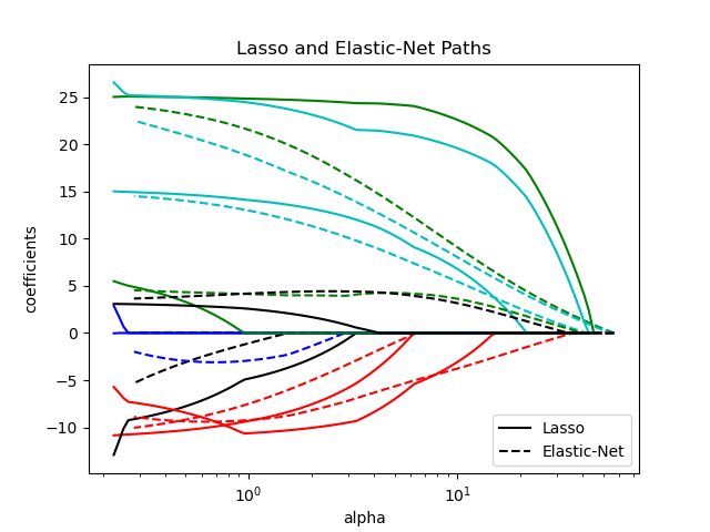
Compare Lasso and Elastic Net
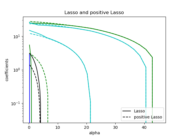
Compare Lasso with positive Lasso
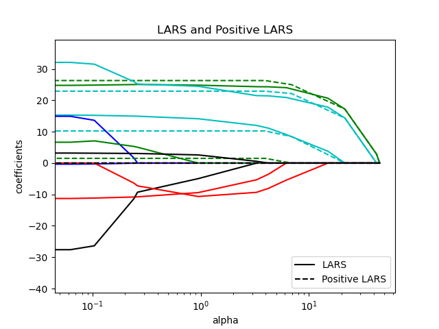
Compare LARS and Positive LARS
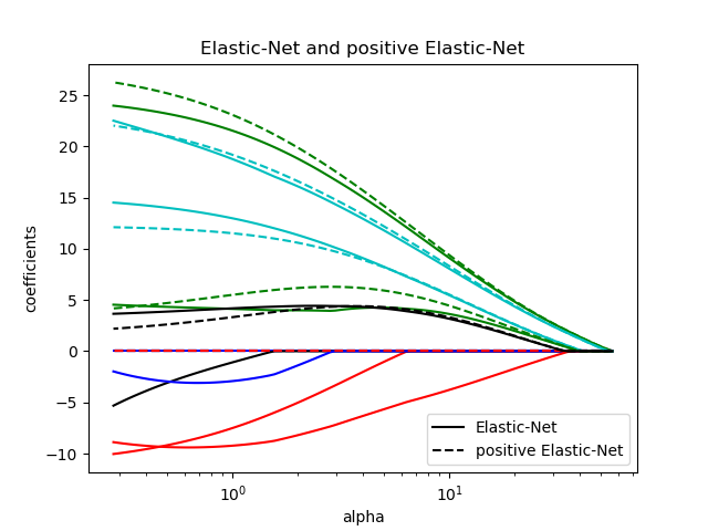
Compare Elastic Net and positive Elastic Net

Each plot shows how the model coefficients vary as the regularization strength changes, offering insight into the behavior of these models under different constraints.

Computing regularization path using the lasso...
Computing regularization path using the positive lasso...
Computing regularization path using the LARS...
Computing regularization path using the positive LARS...
Computing regularization path using the elastic net...
Computing regularization path using the positive elastic net...

# Authors: The scikit-learn developers
# SPDX-License-Identifier: BSD-3-Clause

from itertools import cycle

import matplotlib.pyplot as plt

from sklearn.datasets import load_diabetes
from sklearn.linear_model import enet_path, lars_path, lasso_path

X, y = load_diabetes(return_X_y=True)
X /= X.std(axis=0)  # Standardize data (easier to set the l1_ratio parameter)

# Compute paths

eps = 5e-3  # the smaller it is the longer is the path

print("Computing regularization path using the lasso...")
alphas_lasso, coefs_lasso, _ = lasso_path(X, y, eps=eps)

print("Computing regularization path using the positive lasso...")
alphas_positive_lasso, coefs_positive_lasso, _ = lasso_path(
    X, y, eps=eps, positive=True
)

print("Computing regularization path using the LARS...")
alphas_lars, _, coefs_lars = lars_path(X, y, method="lasso")

print("Computing regularization path using the positive LARS...")
alphas_positive_lars, _, coefs_positive_lars = lars_path(
    X, y, method="lasso", positive=True
)

print("Computing regularization path using the elastic net...")
alphas_enet, coefs_enet, _ = enet_path(X, y, eps=eps, l1_ratio=0.8)

print("Computing regularization path using the positive elastic net...")
alphas_positive_enet, coefs_positive_enet, _ = enet_path(
    X, y, eps=eps, l1_ratio=0.8, positive=True
)

# Display results

plt.figure(1)
colors = cycle(["b", "r", "g", "c", "k"])
for coef_lasso, coef_lars, c in zip(coefs_lasso, coefs_lars, colors):
    l1 = plt.semilogx(alphas_lasso, coef_lasso, c=c)
    l2 = plt.semilogx(alphas_lars, coef_lars, linestyle="--", c=c)

plt.xlabel("alpha")
plt.ylabel("coefficients")
plt.title("Lasso and LARS Paths")
plt.legend((l1[-1], l2[-1]), ("Lasso", "LARS"), loc="lower right")
plt.axis("tight")

plt.figure(2)
colors = cycle(["b", "r", "g", "c", "k"])
for coef_l, coef_e, c in zip(coefs_lasso, coefs_enet, colors):
    l1 = plt.semilogx(alphas_lasso, coef_l, c=c)
    l2 = plt.semilogx(alphas_enet, coef_e, linestyle="--", c=c)

plt.xlabel("alpha")
plt.ylabel("coefficients")
plt.title("Lasso and Elastic-Net Paths")
plt.legend((l1[-1], l2[-1]), ("Lasso", "Elastic-Net"), loc="lower right")
plt.axis("tight")


plt.figure(3)
for coef_l, coef_pl, c in zip(coefs_lasso, coefs_positive_lasso, colors):
    l1 = plt.semilogy(alphas_lasso, coef_l, c=c)
    l2 = plt.semilogy(alphas_positive_lasso, coef_pl, linestyle="--", c=c)

plt.xlabel("alpha")
plt.ylabel("coefficients")
plt.title("Lasso and positive Lasso")
plt.legend((l1[-1], l2[-1]), ("Lasso", "positive Lasso"), loc="lower right")
plt.axis("tight")


plt.figure(4)
colors = cycle(["b", "r", "g", "c", "k"])
for coef_lars, coef_positive_lars, c in zip(coefs_lars, coefs_positive_lars, colors):
    l1 = plt.semilogx(alphas_lars, coef_lars, c=c)
    l2 = plt.semilogx(alphas_positive_lars, coef_positive_lars, linestyle="--", c=c)

plt.xlabel("alpha")
plt.ylabel("coefficients")
plt.title("LARS and Positive LARS")
plt.legend((l1[-1], l2[-1]), ("LARS", "Positive LARS"), loc="lower right")
plt.axis("tight")

plt.figure(5)
for coef_e, coef_pe, c in zip(coefs_enet, coefs_positive_enet, colors):
    l1 = plt.semilogx(alphas_enet, coef_e, c=c)
    l2 = plt.semilogx(alphas_positive_enet, coef_pe, linestyle="--", c=c)

plt.xlabel("alpha")
plt.ylabel("coefficients")
plt.title("Elastic-Net and positive Elastic-Net")
plt.legend((l1[-1], l2[-1]), ("Elastic-Net", "positive Elastic-Net"), loc="lower right")
plt.axis("tight")
plt.show()