Note
Go to the end to download the full example code or to run this example in your browser via JupyterLite or Binder.
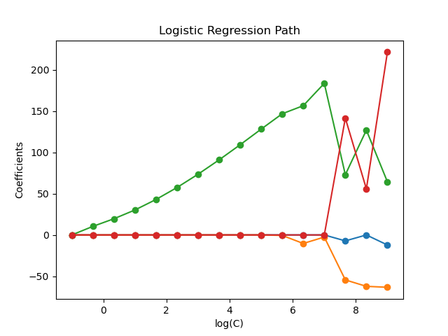
Regularization path of L1- Logistic Regression#
Train l1-penalized logistic regression models on a binary classification problem derived from the Iris dataset.
The models are ordered from strongest regularized to least regularized. The 4 coefficients of the models are collected and plotted as a “regularization path”: on the left-hand side of the figure (strong regularizers), all the coefficients are exactly 0. When regularization gets progressively looser, coefficients can get non-zero values one after the other.
Here we choose the liblinear solver because it can efficiently optimize for the Logistic Regression loss with a non-smooth, sparsity inducing l1 penalty.
Also note that we set a low value for the tolerance to make sure that the model has converged before collecting the coefficients.
We also use warm_start=True which means that the coefficients of the models are reused to initialize the next model fit to speed-up the computation of the full-path.
# Authors: The scikit-learn developers
# SPDX-License-Identifier: BSD-3-Clause
Load data#
from sklearn import datasets

iris = datasets.load_iris()
X = iris.data
y = iris.target
feature_names = iris.feature_names
Here we remove the third class to make the problem a binary classification
X = X[y != 2]
y = y[y != 2]
Compute regularization path#
import numpy as np

from sklearn.linear_model import LogisticRegression
from sklearn.pipeline import make_pipeline
from sklearn.preprocessing import StandardScaler
from sklearn.svm import l1_min_c

cs = l1_min_c(X, y, loss="log") * np.logspace(0, 1, 16)
Create a pipeline with StandardScaler and LogisticRegression, to normalize
the data before fitting a linear model, in order to speed-up convergence and
make the coefficients comparable. Also, as a side effect, since the data is now
centered around 0, we don’t need to fit an intercept.
clf = make_pipeline(
    StandardScaler(),
    LogisticRegression(
        l1_ratio=1,
        solver="liblinear",
        tol=1e-6,
        max_iter=int(1e6),
        warm_start=True,
        fit_intercept=False,
    ),
)
coefs_ = []
for c in cs:
    clf.set_params(logisticregression__C=c)
    clf.fit(X, y)
    coefs_.append(clf["logisticregression"].coef_.ravel().copy())

coefs_ = np.array(coefs_)
Plot regularization path#
import matplotlib.pyplot as plt

# Colorblind-friendly palette (IBM Color Blind Safe palette)
colors = ["#648FFF", "#785EF0", "#DC267F", "#FE6100"]

plt.figure(figsize=(10, 6))
for i in range(coefs_.shape[1]):
    plt.semilogx(cs, coefs_[:, i], marker="o", color=colors[i], label=feature_names[i])

ymin, ymax = plt.ylim()
plt.xlabel("C")
plt.ylabel("Coefficients")
plt.title("Logistic Regression Path")
plt.legend()
plt.axis("tight")
plt.show()
Total running time of the script: (0 minutes 0.218 seconds)
Related examples
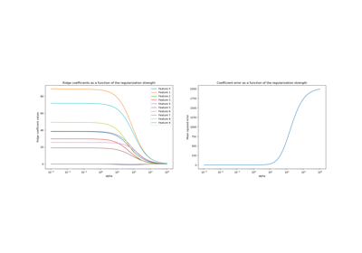
Ridge coefficients as a function of the L2 Regularization
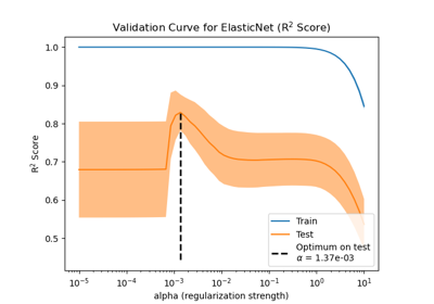
Effect of model regularization on training and test error
Plot Ridge coefficients as a function of the regularization