Note
Go to the end to download the full example code or to run this example in your browser via JupyterLite or Binder.
Gaussian Processes regression: basic introductory example#
A simple one-dimensional regression example computed in two different ways:
A noise-free case
A noisy case with known noise-level per datapoint
In both cases, the kernel’s parameters are estimated using the maximum likelihood principle.
The figures illustrate the interpolating property of the Gaussian Process model as well as its probabilistic nature in the form of a pointwise 95% confidence interval.
Note that alpha is a parameter to control the strength of the Tikhonov
regularization on the assumed training points’ covariance matrix.
# Authors: The scikit-learn developers
# SPDX-License-Identifier: BSD-3-Clause
Dataset generation#
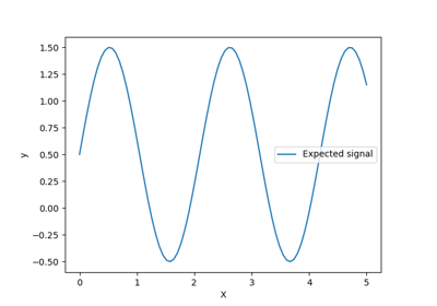
We will start by generating a synthetic dataset. The true generative process is defined as \(f(x) = x \sin(x)\).
import numpy as np

X = np.linspace(start=0, stop=10, num=1_000).reshape(-1, 1)
y = np.squeeze(X * np.sin(X))
import matplotlib.pyplot as plt

plt.plot(X, y, label=r"$f(x) = x \sin(x)$", linestyle="dotted")
plt.legend()
plt.xlabel("$x$")
plt.ylabel("$f(x)$")
_ = plt.title("True generative process")
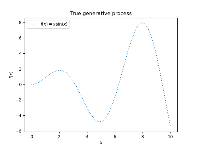
We will use this dataset in the next experiment to illustrate how Gaussian Process regression is working.
Example with noise-free target#
In this first example, we will use the true generative process without adding any noise. For training the Gaussian Process regression, we will only select few samples.
rng = np.random.RandomState(1)
training_indices = rng.choice(np.arange(y.size), size=6, replace=False)
X_train, y_train = X[training_indices], y[training_indices]
Now, we fit a Gaussian process on these few training data samples. We will use a radial basis function (RBF) kernel and a constant parameter to fit the amplitude.
from sklearn.gaussian_process import GaussianProcessRegressor
from sklearn.gaussian_process.kernels import RBF

kernel = 1 * RBF(length_scale=1.0, length_scale_bounds=(1e-2, 1e2))
gaussian_process = GaussianProcessRegressor(kernel=kernel, n_restarts_optimizer=9)
gaussian_process.fit(X_train, y_train)
gaussian_process.kernel_
5.02**2 * RBF(length_scale=1.43)
After fitting our model, we see that the hyperparameters of the kernel have been optimized. Now, we will use our kernel to compute the mean prediction of the full dataset and plot the 95% confidence interval.
mean_prediction, std_prediction = gaussian_process.predict(X, return_std=True)

plt.plot(X, y, label=r"$f(x) = x \sin(x)$", linestyle="dotted")
plt.scatter(X_train, y_train, label="Observations")
plt.plot(X, mean_prediction, label="Mean prediction")
plt.fill_between(
    X.ravel(),
    mean_prediction - 1.96 * std_prediction,
    mean_prediction + 1.96 * std_prediction,
    alpha=0.5,
    label=r"95% confidence interval",
)
plt.legend()
plt.xlabel("$x$")
plt.ylabel("$f(x)$")
_ = plt.title("Gaussian process regression on noise-free dataset")
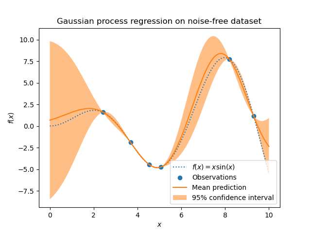
We see that for a prediction made on a data point close to the one from the training set, the 95% confidence has a small amplitude. Whenever a sample falls far from training data, our model’s prediction is less accurate and the model prediction is less precise (higher uncertainty).
Example with noisy targets#
We can repeat a similar experiment adding an additional noise to the target this time. It will allow seeing the effect of the noise on the fitted model.
We add some random Gaussian noise to the target with an arbitrary standard deviation.
noise_std = 0.75
y_train_noisy = y_train + rng.normal(loc=0.0, scale=noise_std, size=y_train.shape)
We create a similar Gaussian process model. In addition to the kernel, this
time, we specify the parameter alpha which can be interpreted as the
variance of a Gaussian noise.
gaussian_process = GaussianProcessRegressor(
    kernel=kernel, alpha=noise_std**2, n_restarts_optimizer=9
)
gaussian_process.fit(X_train, y_train_noisy)
mean_prediction, std_prediction = gaussian_process.predict(X, return_std=True)
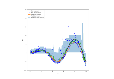
Let’s plot the mean prediction and the uncertainty region as before.
plt.plot(X, y, label=r"$f(x) = x \sin(x)$", linestyle="dotted")
plt.errorbar(
    X_train,
    y_train_noisy,
    noise_std,
    linestyle="None",
    color="tab:blue",
    marker=".",
    markersize=10,
    label="Observations",
)
plt.plot(X, mean_prediction, label="Mean prediction")
plt.fill_between(
    X.ravel(),
    mean_prediction - 1.96 * std_prediction,
    mean_prediction + 1.96 * std_prediction,
    color="tab:orange",
    alpha=0.5,
    label=r"95% confidence interval",
)
plt.legend()
plt.xlabel("$x$")
plt.ylabel("$f(x)$")
_ = plt.title("Gaussian process regression on a noisy dataset")
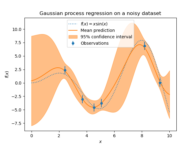
The noise affects the predictions close to the training samples: the predictive uncertainty near to the training samples is larger because we explicitly model a given level target noise independent of the input variable.
Total running time of the script: (0 minutes 0.439 seconds)
Related examples
Comparison of kernel ridge and Gaussian process regression
Ability of Gaussian process regression (GPR) to estimate data noise-level
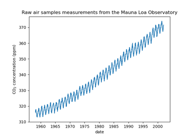
Forecasting of CO2 level on Mona Loa dataset using Gaussian process regression (GPR)
Prediction Intervals for Gradient Boosting Regression
