Evaluation of outlier detection estimators

This example compares two outlier detection algorithms, namely Local Outlier Factor (LOF) and Isolation Forest (IForest), on real-world datasets available in sklearn.datasets. The goal is to show that different algorithms perform well on different datasets and contrast their training speed and sensitivity to hyperparameters.

The algorithms are trained (without labels) on the whole dataset assumed to contain outliers.

1. The ROC curves are computed using knowledge of the ground-truth labels and displayed using RocCurveDisplay.

2. The performance is assessed in terms of the ROC-AUC.

# Author: Pharuj Rajborirug <pharuj.ra@kmitl.ac.th>
#         Arturo Amor <david-arturo.amor-quiroz@inria.fr>
# License: BSD 3 clause

Dataset preprocessing and model training

Different outlier detection models require different preprocessing. In the presence of categorical variables, OrdinalEncoder is often a good strategy for tree-based models such as IsolationForest, whereas neighbors-based models such as LocalOutlierFactor would be impacted by the ordering induced by ordinal encoding. To avoid inducing an ordering, on should rather use OneHotEncoder.

Neighbors-based models may also require scaling of the numerical features (see for instance Effect of rescaling on a k-neighbors models). In the presence of outliers, a good option is to use a RobustScaler.

from sklearn.compose import ColumnTransformer
from sklearn.ensemble import IsolationForest
from sklearn.neighbors import LocalOutlierFactor
from sklearn.pipeline import make_pipeline
from sklearn.preprocessing import (
    OneHotEncoder,
    OrdinalEncoder,
    RobustScaler,
)


def make_estimator(name, categorical_columns=None, iforest_kw=None, lof_kw=None):
    """Create an outlier detection estimator based on its name."""
    if name == "LOF":
        outlier_detector = LocalOutlierFactor(**(lof_kw or {}))
        if categorical_columns is None:
            preprocessor = RobustScaler()
        else:
            preprocessor = ColumnTransformer(
                transformers=[("categorical", OneHotEncoder(), categorical_columns)],
                remainder=RobustScaler(),
            )
    else:  # name == "IForest"
        outlier_detector = IsolationForest(**(iforest_kw or {}))
        if categorical_columns is None:
            preprocessor = None
        else:
            ordinal_encoder = OrdinalEncoder(
                handle_unknown="use_encoded_value", unknown_value=-1
            )
            preprocessor = ColumnTransformer(
                transformers=[
                    ("categorical", ordinal_encoder, categorical_columns),
                ],
                remainder="passthrough",
            )

    return make_pipeline(preprocessor, outlier_detector)

The following fit_predict function returns the average outlier score of X.

from time import perf_counter


def fit_predict(estimator, X):
    tic = perf_counter()
    if estimator[-1].__class__.__name__ == "LocalOutlierFactor":
        estimator.fit(X)
        y_pred = estimator[-1].negative_outlier_factor_
    else:  # "IsolationForest"
        y_pred = estimator.fit(X).decision_function(X)
    toc = perf_counter()
    print(f"Duration for {model_name}: {toc - tic:.2f} s")
    return y_pred

On the rest of the example we process one dataset per section. After loading the data, the targets are modified to consist of two classes: 0 representing inliers and 1 representing outliers. Due to computational constraints of the scikit-learn documentation, the sample size of some datasets is reduced using a stratified train_test_split.

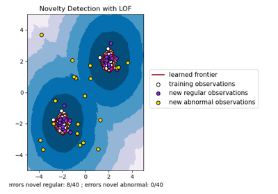
Furthermore, we set n_neighbors to match the expected number of anomalies expected_n_anomalies = n_samples * expected_anomaly_fraction. This is a good heuristic as long as the proportion of outliers is not very low, the reason being that n_neighbors should be at least greater than the number of samples in the less populated cluster (see Outlier detection with Local Outlier Factor (LOF)).

KDDCup99 - SA dataset

The Kddcup 99 dataset was generated using a closed network and hand-injected attacks. The SA dataset is a subset of it obtained by simply selecting all the normal data and an anomaly proportion of around 3%.

import numpy as np

from sklearn.datasets import fetch_kddcup99
from sklearn.model_selection import train_test_split

X, y = fetch_kddcup99(
    subset="SA", percent10=True, random_state=42, return_X_y=True, as_frame=True
)
y = (y != b"normal.").astype(np.int32)
X, _, y, _ = train_test_split(X, y, train_size=0.1, stratify=y, random_state=42)

n_samples, anomaly_frac = X.shape[0], y.mean()
print(f"{n_samples} datapoints with {y.sum()} anomalies ({anomaly_frac:.02%})")

10065 datapoints with 338 anomalies (3.36%)

The SA dataset contains 41 features out of which 3 are categorical: “protocol_type”, “service” and “flag”.

y_true = {}
y_pred = {"LOF": {}, "IForest": {}}
model_names = ["LOF", "IForest"]
cat_columns = ["protocol_type", "service", "flag"]

y_true["KDDCup99 - SA"] = y
for model_name in model_names:
    model = make_estimator(
        name=model_name,
        categorical_columns=cat_columns,
        lof_kw={"n_neighbors": int(n_samples * anomaly_frac)},
        iforest_kw={"random_state": 42},
    )
    y_pred[model_name]["KDDCup99 - SA"] = fit_predict(model, X)

Duration for LOF: 1.95 s
Duration for IForest: 0.28 s

Forest covertypes dataset

The Forest covertypes is a multiclass dataset where the target is the dominant species of tree in a given patch of forest. It contains 54 features, some of which (“Wilderness_Area” and “Soil_Type”) are already binary encoded. Though originally meant as a classification task, one can regard inliers as samples encoded with label 2 and outliers as those with label 4.

from sklearn.datasets import fetch_covtype

X, y = fetch_covtype(return_X_y=True, as_frame=True)
s = (y == 2) + (y == 4)
X = X.loc[s]
y = y.loc[s]
y = (y != 2).astype(np.int32)

X, _, y, _ = train_test_split(X, y, train_size=0.05, stratify=y, random_state=42)
X_forestcover = X  # save X for later use

n_samples, anomaly_frac = X.shape[0], y.mean()
print(f"{n_samples} datapoints with {y.sum()} anomalies ({anomaly_frac:.02%})")

14302 datapoints with 137 anomalies (0.96%)

y_true["forestcover"] = y
for model_name in model_names:
    model = make_estimator(
        name=model_name,
        lof_kw={"n_neighbors": int(n_samples * anomaly_frac)},
        iforest_kw={"random_state": 42},
    )
    y_pred[model_name]["forestcover"] = fit_predict(model, X)

Duration for LOF: 1.91 s
Duration for IForest: 0.21 s

Ames Housing dataset

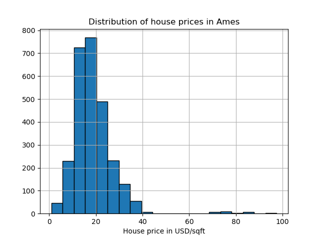
The Ames housing dataset is originally a regression dataset where the target are sales prices of houses in Ames, Iowa. Here we convert it into an outlier detection problem by regarding houses with price over 70 USD/sqft. To make the problem easier, we drop intermediate prices between 40 and 70 USD/sqft.

import matplotlib.pyplot as plt

from sklearn.datasets import fetch_openml

X, y = fetch_openml(name="ames_housing", version=1, return_X_y=True, as_frame=True)
y = y.div(X["Lot_Area"])

# None values in pandas 1.5.1 were mapped to np.nan in pandas 2.0.1
X["Misc_Feature"] = X["Misc_Feature"].cat.add_categories("NoInfo").fillna("NoInfo")
X["Mas_Vnr_Type"] = X["Mas_Vnr_Type"].cat.add_categories("NoInfo").fillna("NoInfo")

X.drop(columns="Lot_Area", inplace=True)
mask = (y < 40) | (y > 70)
X = X.loc[mask]
y = y.loc[mask]
y.hist(bins=20, edgecolor="black")
plt.xlabel("House price in USD/sqft")
_ = plt.title("Distribution of house prices in Ames")

y = (y > 70).astype(np.int32)

n_samples, anomaly_frac = X.shape[0], y.mean()
print(f"{n_samples} datapoints with {y.sum()} anomalies ({anomaly_frac:.02%})")

2714 datapoints with 30 anomalies (1.11%)

The dataset contains 46 categorical features. In this case it is easier use a make_column_selector to find them instead of passing a list made by hand.

from sklearn.compose import make_column_selector as selector

categorical_columns_selector = selector(dtype_include="category")
cat_columns = categorical_columns_selector(X)

y_true["ames_housing"] = y
for model_name in model_names:
    model = make_estimator(
        name=model_name,
        categorical_columns=cat_columns,
        lof_kw={"n_neighbors": int(n_samples * anomaly_frac)},
        iforest_kw={"random_state": 42},
    )
    y_pred[model_name]["ames_housing"] = fit_predict(model, X)

Duration for LOF: 0.84 s
Duration for IForest: 0.21 s

Cardiotocography dataset

The Cardiotocography dataset is a multiclass dataset of fetal cardiotocograms, the classes being the fetal heart rate (FHR) pattern encoded with labels from 1 to 10. Here we set class 3 (the minority class) to represent the outliers. It contains 30 numerical features, some of which are binary encoded and some are continuous.

X, y = fetch_openml(name="cardiotocography", version=1, return_X_y=True, as_frame=False)
X_cardiotocography = X  # save X for later use
s = y == "3"
y = s.astype(np.int32)

n_samples, anomaly_frac = X.shape[0], y.mean()
print(f"{n_samples} datapoints with {y.sum()} anomalies ({anomaly_frac:.02%})")

2126 datapoints with 53 anomalies (2.49%)

y_true["cardiotocography"] = y
for model_name in model_names:
    model = make_estimator(
        name=model_name,
        lof_kw={"n_neighbors": int(n_samples * anomaly_frac)},
        iforest_kw={"random_state": 42},
    )
    y_pred[model_name]["cardiotocography"] = fit_predict(model, X)

Duration for LOF: 0.06 s
Duration for IForest: 0.13 s

Plot and interpret results

The algorithm performance relates to how good the true positive rate (TPR) is at low value of the false positive rate (FPR). The best algorithms have the curve on the top-left of the plot and the area under curve (AUC) close to 1. The diagonal dashed line represents a random classification of outliers and inliers.

import math

from sklearn.metrics import RocCurveDisplay

cols = 2
pos_label = 0  # mean 0 belongs to positive class
datasets_names = y_true.keys()
rows = math.ceil(len(datasets_names) / cols)

fig, axs = plt.subplots(nrows=rows, ncols=cols, squeeze=False, figsize=(10, rows * 4))

for ax, dataset_name in zip(axs.ravel(), datasets_names):
    for model_idx, model_name in enumerate(model_names):
        display = RocCurveDisplay.from_predictions(
            y_true[dataset_name],
            y_pred[model_name][dataset_name],
            pos_label=pos_label,
            name=model_name,
            ax=ax,
            plot_chance_level=(model_idx == len(model_names) - 1),
            chance_level_kw={"linestyle": ":"},
        )
    ax.set_title(dataset_name)
_ = plt.tight_layout(pad=2.0)  # spacing between subplots

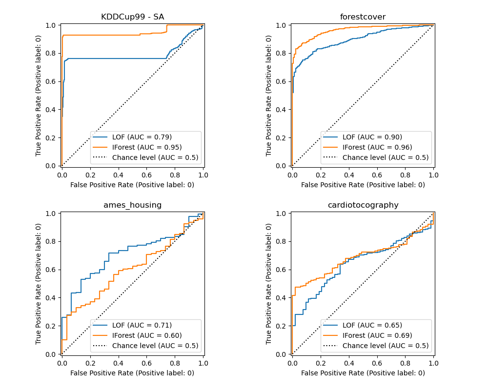
We observe that once the number of neighbors is tuned, LOF and IForest perform similarly in terms of ROC AUC for the forestcover and cardiotocography datasets. The score for IForest is slightly better for the SA dataset and LOF performs considerably better on the Ames housing dataset than IForest.

Recall however that Isolation Forest tends to train much faster than LOF on datasets with a large number of samples. LOF needs to compute pairwise distances to find nearest neighbors, which has a quadratic complexity with respect to the number of observations. This can make this method prohibitive on large datasets.

Ablation study

In this section we explore the impact of the hyperparameter n_neighbors and the choice of scaling the numerical variables on the LOF model. Here we use the Forest covertypes dataset as the binary encoded categories introduce a natural scale of euclidean distances between 0 and 1. We then want a scaling method to avoid granting a privilege to non-binary features and that is robust enough to outliers so that the task of finding them does not become too difficult.

X = X_forestcover
y = y_true["forestcover"]

n_samples = X.shape[0]
n_neighbors_list = (n_samples * np.array([0.2, 0.02, 0.01, 0.001])).astype(np.int32)
model = make_pipeline(RobustScaler(), LocalOutlierFactor())

linestyles = ["solid", "dashed", "dashdot", ":", (5, (10, 3))]

fig, ax = plt.subplots()
for model_idx, (linestyle, n_neighbors) in enumerate(zip(linestyles, n_neighbors_list)):
    model.set_params(localoutlierfactor__n_neighbors=n_neighbors)
    model.fit(X)
    y_pred = model[-1].negative_outlier_factor_
    display = RocCurveDisplay.from_predictions(
        y,
        y_pred,
        pos_label=pos_label,
        name=f"n_neighbors = {n_neighbors}",
        ax=ax,
        plot_chance_level=(model_idx == len(n_neighbors_list) - 1),
        chance_level_kw={"linestyle": (0, (1, 10))},
        linestyle=linestyle,
        linewidth=2,
    )
_ = ax.set_title("RobustScaler with varying n_neighbors\non forestcover dataset")

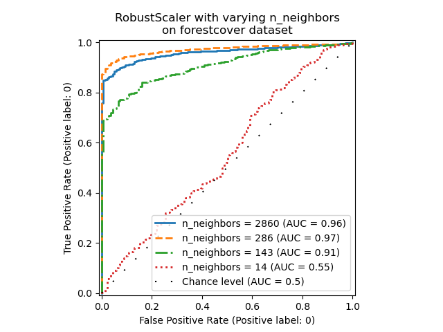
We observe that the number of neighbors has a big impact on the performance of the model. If one has access to (at least some) ground truth labels, it is then important to tune n_neighbors accordingly. A convenient way to do so is to explore values for n_neighbors of the order of magnitud of the expected contamination.

from sklearn.preprocessing import MinMaxScaler, SplineTransformer, StandardScaler

preprocessor_list = [
    None,
    RobustScaler(),
    StandardScaler(),
    MinMaxScaler(),
    SplineTransformer(),
]
expected_anomaly_fraction = 0.02
lof = LocalOutlierFactor(n_neighbors=int(n_samples * expected_anomaly_fraction))

fig, ax = plt.subplots()
for model_idx, (linestyle, preprocessor) in enumerate(
    zip(linestyles, preprocessor_list)
):
    model = make_pipeline(preprocessor, lof)
    model.fit(X)
    y_pred = model[-1].negative_outlier_factor_
    display = RocCurveDisplay.from_predictions(
        y,
        y_pred,
        pos_label=pos_label,
        name=str(preprocessor).split("(")[0],
        ax=ax,
        plot_chance_level=(model_idx == len(preprocessor_list) - 1),
        chance_level_kw={"linestyle": (0, (1, 10))},
        linestyle=linestyle,
        linewidth=2,
    )
_ = ax.set_title("Fixed n_neighbors with varying preprocessing\non forestcover dataset")

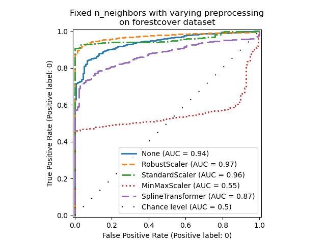
On the one hand, RobustScaler scales each feature independently by using the interquartile range (IQR) by default, which is the range between the 25th and 75th percentiles of the data. It centers the data by subtracting the median and then scale it by dividing by the IQR. The IQR is robust to outliers: the median and interquartile range are less affected by extreme values than the range, the mean and the standard deviation. Furthermore, RobustScaler does not squash marginal outlier values, contrary to StandardScaler.

On the other hand, MinMaxScaler scales each feature individually such that its range maps into the range between zero and one. If there are outliers in the data, they can skew it towards either the minimum or maximum values, leading to a completely different distribution of data with large marginal outliers: all non-outlier values can be collapsed almost together as a result.

We also evaluated no preprocessing at all (by passing None to the pipeline), StandardScaler and SplineTransformer. Please refer to their respective documentation for more details.

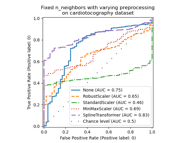
Note that the optimal preprocessing depends on the dataset, as shown below:

X = X_cardiotocography
y = y_true["cardiotocography"]

n_samples, expected_anomaly_fraction = X.shape[0], 0.025
lof = LocalOutlierFactor(n_neighbors=int(n_samples * expected_anomaly_fraction))

fig, ax = plt.subplots()
for model_idx, (linestyle, preprocessor) in enumerate(
    zip(linestyles, preprocessor_list)
):
    model = make_pipeline(preprocessor, lof)
    model.fit(X)
    y_pred = model[-1].negative_outlier_factor_
    display = RocCurveDisplay.from_predictions(
        y,
        y_pred,
        pos_label=pos_label,
        name=str(preprocessor).split("(")[0],
        ax=ax,
        plot_chance_level=(model_idx == len(preprocessor_list) - 1),
        chance_level_kw={"linestyle": (0, (1, 10))},
        linestyle=linestyle,
        linewidth=2,
    )
ax.set_title(
    "Fixed n_neighbors with varying preprocessing\non cardiotocography dataset"
)
plt.show()

Related examples

Outlier detection with Local Outlier Factor (LOF)

Outlier detection with Local Outlier Factor (LOF)

Comparing anomaly detection algorithms for outlier detection on toy datasets

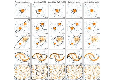
Comparing anomaly detection algorithms for outlier detection on toy datasets

Compare the effect of different scalers on data with outliers

Compare the effect of different scalers on data with outliers

Novelty detection with Local Outlier Factor (LOF)

Novelty detection with Local Outlier Factor (LOF)

Combine predictors using stacking

Combine predictors using stacking