Note
Go to the end to download the full example code or to run this example in your browser via JupyterLite or Binder.
Curve Fitting with Bayesian Ridge Regression#
Computes a Bayesian Ridge Regression of Sinusoids.
See Bayesian Ridge Regression for more information on the regressor.
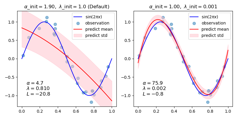
In general, when fitting a curve with a polynomial by Bayesian ridge regression, the selection of initial values of the regularization parameters (alpha, lambda) may be important. This is because the regularization parameters are determined by an iterative procedure that depends on initial values.
In this example, the sinusoid is approximated by a polynomial using different pairs of initial values.
When starting from the default values (alpha_init = 1.90, lambda_init = 1.), the bias of the resulting curve is large, and the variance is small. So, lambda_init should be relatively small (1.e-3) so as to reduce the bias.
Also, by evaluating log marginal likelihood (L) of these models, we can determine which one is better. It can be concluded that the model with larger L is more likely.
# Authors: The scikit-learn developers
# SPDX-License-Identifier: BSD-3-Clause
Generate sinusoidal data with noise#
import numpy as np


def func(x):
    return np.sin(2 * np.pi * x)


size = 25
rng = np.random.RandomState(1234)
x_train = rng.uniform(0.0, 1.0, size)
y_train = func(x_train) + rng.normal(scale=0.1, size=size)
x_test = np.linspace(0.0, 1.0, 100)
Fit by cubic polynomial#
from sklearn.linear_model import BayesianRidge

n_order = 3
X_train = np.vander(x_train, n_order + 1, increasing=True)
X_test = np.vander(x_test, n_order + 1, increasing=True)
reg = BayesianRidge(tol=1e-6, fit_intercept=False, compute_score=True)
Plot the true and predicted curves with log marginal likelihood (L)#
import matplotlib.pyplot as plt

fig, axes = plt.subplots(1, 2, figsize=(8, 4))
for i, ax in enumerate(axes):
    # Bayesian ridge regression with different initial value pairs
    if i == 0:
        init = [1 / np.var(y_train), 1.0]  # Default values
    elif i == 1:
        init = [1.0, 1e-3]
        reg.set_params(alpha_init=init[0], lambda_init=init[1])
    reg.fit(X_train, y_train)
    ymean, ystd = reg.predict(X_test, return_std=True)

    ax.plot(x_test, func(x_test), color="blue", label="sin($2\\pi x$)")
    ax.scatter(x_train, y_train, s=50, alpha=0.5, label="observation")
    ax.plot(x_test, ymean, color="red", label="predict mean")
    ax.fill_between(
        x_test, ymean - ystd, ymean + ystd, color="pink", alpha=0.5, label="predict std"
    )
    ax.set_ylim(-1.3, 1.3)
    ax.legend()
    title = "$\\alpha$_init$={:.2f},\\ \\lambda$_init$={}$".format(init[0], init[1])
    if i == 0:
        title += " (Default)"
    ax.set_title(title, fontsize=12)
    text = "$\\alpha={:.1f}$\n$\\lambda={:.3f}$\n$L={:.1f}$".format(
        reg.alpha_, reg.lambda_, reg.scores_[-1]
    )
    ax.text(0.05, -1.0, text, fontsize=12)

plt.tight_layout()
plt.show()
Total running time of the script: (0 minutes 0.501 seconds)
Related examples
Using KBinsDiscretizer to discretize continuous features
Empirical evaluation of the impact of k-means initialization