Note
Go to the end to download the full example code or to run this example in your browser via JupyterLite or Binder.
Outlier detection on a real data set#
This example illustrates the need for robust covariance estimation on a real data set. It is useful both for outlier detection and for a better understanding of the data structure.
We selected two sets of two variables from the Wine data set as an illustration of what kind of analysis can be done with several outlier detection tools. For the purpose of visualization, we are working with two-dimensional examples, but one should be aware that things are not so trivial in high-dimension, as it will be pointed out.
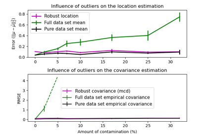
In both examples below, the main result is that the empirical covariance estimate, as a non-robust one, is highly influenced by the heterogeneous structure of the observations. Although the robust covariance estimate is able to focus on the main mode of the data distribution, it sticks to the assumption that the data should be Gaussian distributed, yielding some biased estimation of the data structure, but yet accurate to some extent. The One-Class SVM does not assume any parametric form of the data distribution and can therefore model the complex shape of the data much better.
# Authors: The scikit-learn developers
# SPDX-License-Identifier: BSD-3-Clause
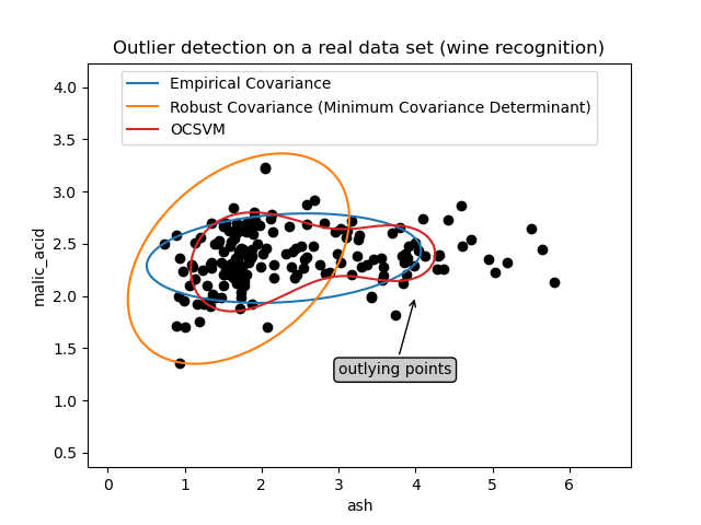
First example#
The first example illustrates how the Minimum Covariance Determinant robust estimator can help concentrate on a relevant cluster when outlying points exist. Here the empirical covariance estimation is skewed by points outside of the main cluster. Of course, some screening tools would have pointed out the presence of two clusters (Support Vector Machines, Gaussian Mixture Models, univariate outlier detection, …). But had it been a high-dimensional example, none of these could be applied that easily.
from sklearn.covariance import EllipticEnvelope
from sklearn.inspection import DecisionBoundaryDisplay
from sklearn.svm import OneClassSVM

estimators = {
    "Empirical Covariance": EllipticEnvelope(support_fraction=1.0, contamination=0.25),
    "Robust Covariance (Minimum Covariance Determinant)": EllipticEnvelope(
        contamination=0.25
    ),
    "OCSVM": OneClassSVM(nu=0.25, gamma=0.35),
}
import matplotlib.lines as mlines
import matplotlib.pyplot as plt

from sklearn.datasets import load_wine

X = load_wine()["data"][:, [1, 2]]  # two clusters

fig, ax = plt.subplots()
colors = ["tab:blue", "tab:orange", "tab:red"]
# Learn a frontier for outlier detection with several classifiers
legend_lines = []
for color, (name, estimator) in zip(colors, estimators.items()):
    estimator.fit(X)
    DecisionBoundaryDisplay.from_estimator(
        estimator,
        X,
        response_method="decision_function",
        plot_method="contour",
        levels=[0],
        colors=color,
        ax=ax,
    )
    legend_lines.append(mlines.Line2D([], [], color=color, label=name))


ax.scatter(X[:, 0], X[:, 1], color="black")
bbox_args = dict(boxstyle="round", fc="0.8")
arrow_args = dict(arrowstyle="->")
ax.annotate(
    "outlying points",
    xy=(4, 2),
    xycoords="data",
    textcoords="data",
    xytext=(3, 1.25),
    bbox=bbox_args,
    arrowprops=arrow_args,
)
ax.legend(handles=legend_lines, loc="upper center")
_ = ax.set(
    xlabel="ash",
    ylabel="malic_acid",
    title="Outlier detection on a real data set (wine recognition)",
)
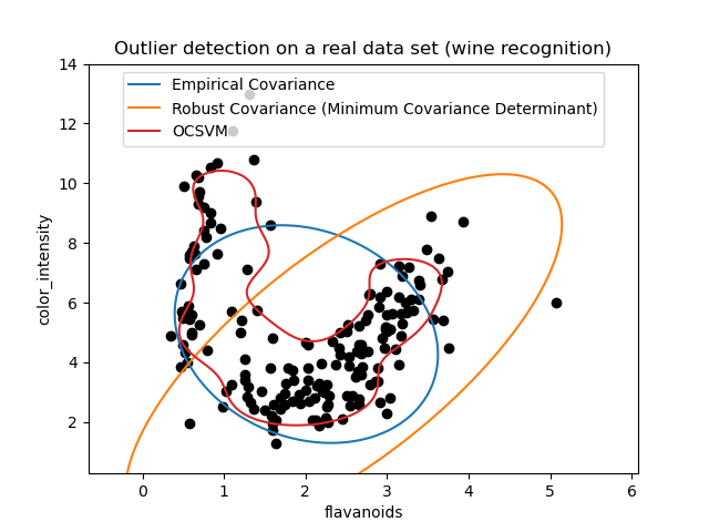
Second example#
The second example shows the ability of the Minimum Covariance Determinant robust estimator of covariance to concentrate on the main mode of the data distribution: the location seems to be well estimated, although the covariance is hard to estimate due to the banana-shaped distribution. Anyway, we can get rid of some outlying observations. The One-Class SVM is able to capture the real data structure, but the difficulty is to adjust its kernel bandwidth parameter so as to obtain a good compromise between the shape of the data scatter matrix and the risk of over-fitting the data.
X = load_wine()["data"][:, [6, 9]]  # "banana"-shaped

fig, ax = plt.subplots()
colors = ["tab:blue", "tab:orange", "tab:red"]
# Learn a frontier for outlier detection with several classifiers
legend_lines = []
for color, (name, estimator) in zip(colors, estimators.items()):
    estimator.fit(X)
    DecisionBoundaryDisplay.from_estimator(
        estimator,
        X,
        response_method="decision_function",
        plot_method="contour",
        levels=[0],
        colors=color,
        ax=ax,
    )
    legend_lines.append(mlines.Line2D([], [], color=color, label=name))


ax.scatter(X[:, 0], X[:, 1], color="black")
ax.legend(handles=legend_lines, loc="upper center")
ax.set(
    xlabel="flavanoids",
    ylabel="color_intensity",
    title="Outlier detection on a real data set (wine recognition)",
)

plt.show()
Total running time of the script: (0 minutes 0.497 seconds)
Related examples
Comparing anomaly detection algorithms for outlier detection on toy datasets
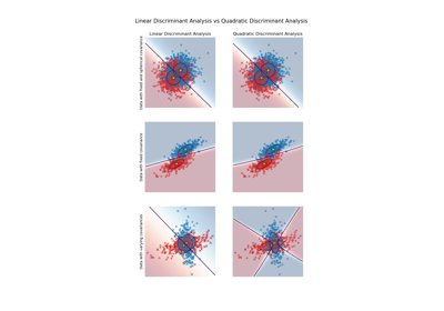
Linear and Quadratic Discriminant Analysis with covariance ellipsoid
