Note

Go to the end to download the full example code. or to run this example in your browser via JupyterLite or Binder

Principal Component Analysis (PCA) on Iris Dataset#

This example shows a well known decomposition technique known as Principal Component Analysis (PCA) on the Iris dataset.

This dataset is made of 4 features: sepal length, sepal width, petal length, petal width. We use PCA to project this 4 feature space into a 3-dimensional space.

# Authors: The scikit-learn developers
# SPDX-License-Identifier: BSD-3-Clause

Loading the Iris dataset#

The Iris dataset is directly available as part of scikit-learn. It can be loaded using the load_iris function. With the default parameters, a Bunch object is returned, containing the data, the target values, the feature names, and the target names.

from sklearn.datasets import load_iris

iris = load_iris(as_frame=True)
print(iris.keys())

dict_keys(['data', 'target', 'frame', 'target_names', 'DESCR', 'feature_names', 'filename', 'data_module'])

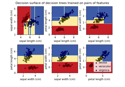
Plot of pairs of features of the Iris dataset#

Let’s first plot the pairs of features of the Iris dataset.

import seaborn as sns

# Rename classes using the iris target names
iris.frame["target"] = iris.target_names[iris.target]
_ = sns.pairplot(iris.frame, hue="target")

Each data point on each scatter plot refers to one of the 150 iris flowers in the dataset, with the color indicating their respective type (Setosa, Versicolor, and Virginica).

You can already see a pattern regarding the Setosa type, which is easily identifiable based on its short and wide sepal. Only considering these two dimensions, sepal width and length, there’s still overlap between the Versicolor and Virginica types.

The diagonal of the plot shows the distribution of each feature. We observe that the petal width and the petal length are the most discriminant features for the three types.

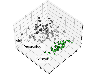
Plot a PCA representation#

Let’s apply a Principal Component Analysis (PCA) to the iris dataset and then plot the irises across the first three PCA dimensions. This will allow us to better differentiate among the three types!

import matplotlib.pyplot as plt

# unused but required import for doing 3d projections with matplotlib < 3.2
import mpl_toolkits.mplot3d  # noqa: F401

from sklearn.decomposition import PCA

fig = plt.figure(1, figsize=(8, 6))
ax = fig.add_subplot(111, projection="3d", elev=-150, azim=110)

X_reduced = PCA(n_components=3).fit_transform(iris.data)
scatter = ax.scatter(
    X_reduced[:, 0],
    X_reduced[:, 1],
    X_reduced[:, 2],
    c=iris.target,
    s=40,
)

ax.set(
    title="First three PCA dimensions",
    xlabel="1st Eigenvector",
    ylabel="2nd Eigenvector",
    zlabel="3rd Eigenvector",
)
ax.xaxis.set_ticklabels([])
ax.yaxis.set_ticklabels([])
ax.zaxis.set_ticklabels([])

# Add a legend
legend1 = ax.legend(
    scatter.legend_elements()[0],
    iris.target_names.tolist(),
    loc="upper right",
    title="Classes",
)
ax.add_artist(legend1)

plt.show()

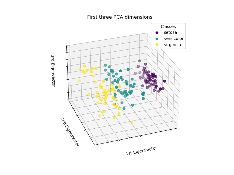
PCA will create 3 new features that are a linear combination of the 4 original features. In addition, this transformation maximizes the variance. With this transformation, we see that we can identify each species using only the first feature (i.e., first eigenvector).

Total running time of the script: (0 minutes 2.740 seconds)