Note

Go to the end to download the full example code or to run this example in your browser via JupyterLite or Binder.

Density Estimation for a Gaussian mixture#

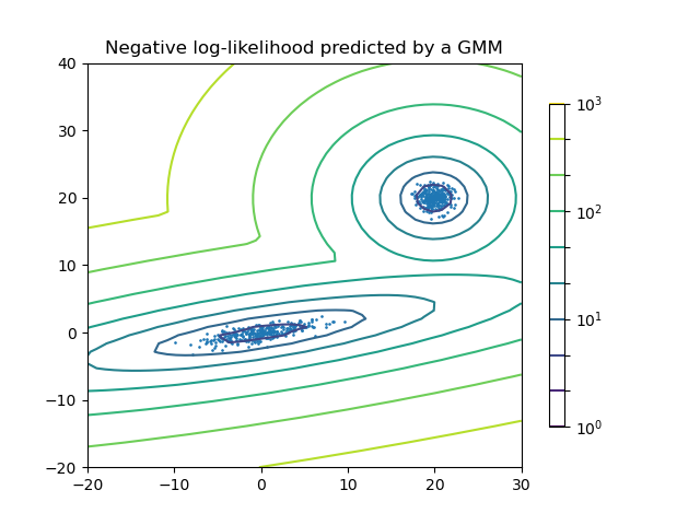
Plot the density estimation of a mixture of two Gaussians. Data is generated from two Gaussians with different centers and covariance matrices.

Negative log-likelihood predicted by a GMM

# Authors: The scikit-learn developers
# SPDX-License-Identifier: BSD-3-Clause

import matplotlib.pyplot as plt
import numpy as np
from matplotlib.colors import LogNorm

from sklearn import mixture

n_samples = 300

# generate random sample, two components
np.random.seed(0)

# generate spherical data centered on (20, 20)
shifted_gaussian = np.random.randn(n_samples, 2) + np.array([20, 20])

# generate zero centered stretched Gaussian data
C = np.array([[0.0, -0.7], [3.5, 0.7]])
stretched_gaussian = np.dot(np.random.randn(n_samples, 2), C)

# concatenate the two datasets into the final training set
X_train = np.vstack([shifted_gaussian, stretched_gaussian])

# fit a Gaussian Mixture Model with two components
clf = mixture.GaussianMixture(n_components=2, covariance_type="full")
clf.fit(X_train)

# display predicted scores by the model as a contour plot
x = np.linspace(-20.0, 30.0)
y = np.linspace(-20.0, 40.0)
X, Y = np.meshgrid(x, y)
XX = np.array([X.ravel(), Y.ravel()]).T
Z = -clf.score_samples(XX)
Z = Z.reshape(X.shape)

CS = plt.contour(
    X, Y, Z, norm=LogNorm(vmin=1.0, vmax=1000.0), levels=np.logspace(0, 3, 10)
)
CB = plt.colorbar(CS, shrink=0.8, extend="both")
plt.scatter(X_train[:, 0], X_train[:, 1], 0.8)

plt.title("Negative log-likelihood predicted by a GMM")
plt.axis("tight")
plt.show()