Note
Go to the end to download the full example code or to run this example in your browser via JupyterLite or Binder.
Release Highlights for scikit-learn 0.23#
We are pleased to announce the release of scikit-learn 0.23! Many bug fixes and improvements were added, as well as some new key features. We detail below a few of the major features of this release. For an exhaustive list of all the changes, please refer to the release notes.
To install the latest version (with pip):
pip install --upgrade scikit-learn
or with conda:
conda install -c conda-forge scikit-learn
Generalized Linear Models, and Poisson loss for gradient boosting#
Long-awaited Generalized Linear Models with non-normal loss functions are now
available. In particular, three new regressors were implemented:
PoissonRegressor,
GammaRegressor, and
TweedieRegressor. The Poisson regressor can be
used to model positive integer counts, or relative frequencies. Read more in
the User Guide. Additionally,
HistGradientBoostingRegressor supports a new
‘poisson’ loss as well.
import numpy as np

from sklearn.ensemble import HistGradientBoostingRegressor
from sklearn.linear_model import PoissonRegressor
from sklearn.model_selection import train_test_split

n_samples, n_features = 1000, 20
rng = np.random.RandomState(0)
X = rng.randn(n_samples, n_features)
# positive integer target correlated with X[:, 5] with many zeros:
y = rng.poisson(lam=np.exp(X[:, 5]) / 2)
X_train, X_test, y_train, y_test = train_test_split(X, y, random_state=rng)
glm = PoissonRegressor()
gbdt = HistGradientBoostingRegressor(loss="poisson", learning_rate=0.01)
glm.fit(X_train, y_train)
gbdt.fit(X_train, y_train)
print(glm.score(X_test, y_test))
print(gbdt.score(X_test, y_test))
0.35776189065725805
0.4366191749596743
Rich visual representation of estimators#
Estimators can now be visualized in notebooks by enabling the
display='diagram' option. This is particularly useful to summarise the
structure of pipelines and other composite estimators, with interactivity to
provide detail. Click on the example image below to expand Pipeline
elements. See Visualizing Composite Estimators for how you can use
this feature.
from sklearn import set_config
from sklearn.compose import make_column_transformer
from sklearn.impute import SimpleImputer
from sklearn.linear_model import LogisticRegression
from sklearn.pipeline import make_pipeline
from sklearn.preprocessing import OneHotEncoder, StandardScaler

set_config(display="diagram")

num_proc = make_pipeline(SimpleImputer(strategy="median"), StandardScaler())

cat_proc = make_pipeline(
    SimpleImputer(strategy="constant", fill_value="missing"),
    OneHotEncoder(handle_unknown="ignore"),
)

preprocessor = make_column_transformer(
    (num_proc, ("feat1", "feat3")), (cat_proc, ("feat0", "feat2"))
)

clf = make_pipeline(preprocessor, LogisticRegression())
clf
Scalability and stability improvements to KMeans#
The KMeans estimator was entirely re-worked, and it
is now significantly faster and more stable. In addition, the Elkan algorithm
is now compatible with sparse matrices. The estimator uses OpenMP based
parallelism instead of relying on joblib, so the n_jobs parameter has no
effect anymore. For more details on how to control the number of threads,
please refer to our Parallelism notes.
import numpy as np
import scipy

from sklearn.cluster import KMeans
from sklearn.datasets import make_blobs
from sklearn.metrics import completeness_score
from sklearn.model_selection import train_test_split

rng = np.random.RandomState(0)
X, y = make_blobs(random_state=rng)
X = scipy.sparse.csr_matrix(X)
X_train, X_test, _, y_test = train_test_split(X, y, random_state=rng)
kmeans = KMeans(n_init="auto").fit(X_train)
print(completeness_score(kmeans.predict(X_test), y_test))
0.7344702338913751
Improvements to the histogram-based Gradient Boosting estimators#
Various improvements were made to
HistGradientBoostingClassifier and
HistGradientBoostingRegressor. On top of the
Poisson loss mentioned above, these estimators now support sample
weights. Also, an automatic early-stopping criterion was added:
early-stopping is enabled by default when the number of samples exceeds 10k.
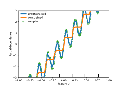
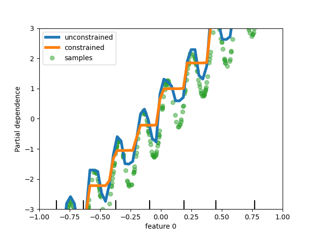
Finally, users can now define monotonic constraints to constrain the predictions based on the variations of
specific features. In the following example, we construct a target that is
generally positively correlated with the first feature, with some noise.
Applying monotoinc constraints allows the prediction to capture the global
effect of the first feature, instead of fitting the noise. For a usecase
example, see Features in Histogram Gradient Boosting Trees.
import numpy as np
from matplotlib import pyplot as plt

from sklearn.ensemble import HistGradientBoostingRegressor

# from sklearn.inspection import plot_partial_dependence
from sklearn.inspection import PartialDependenceDisplay
from sklearn.model_selection import train_test_split

n_samples = 500
rng = np.random.RandomState(0)
X = rng.randn(n_samples, 2)
noise = rng.normal(loc=0.0, scale=0.01, size=n_samples)
y = 5 * X[:, 0] + np.sin(10 * np.pi * X[:, 0]) - noise

gbdt_no_cst = HistGradientBoostingRegressor().fit(X, y)
gbdt_cst = HistGradientBoostingRegressor(monotonic_cst=[1, 0]).fit(X, y)

# plot_partial_dependence has been removed in version 1.2. From 1.2, use
# PartialDependenceDisplay instead.
# disp = plot_partial_dependence(
disp = PartialDependenceDisplay.from_estimator(
    gbdt_no_cst,
    X,
    features=[0],
    feature_names=["feature 0"],
    line_kw={"linewidth": 4, "label": "unconstrained", "color": "tab:blue"},
)
# plot_partial_dependence(
PartialDependenceDisplay.from_estimator(
    gbdt_cst,
    X,
    features=[0],
    line_kw={"linewidth": 4, "label": "constrained", "color": "tab:orange"},
    ax=disp.axes_,
)
disp.axes_[0, 0].plot(
    X[:, 0], y, "o", alpha=0.5, zorder=-1, label="samples", color="tab:green"
)
disp.axes_[0, 0].set_ylim(-3, 3)
disp.axes_[0, 0].set_xlim(-1, 1)
plt.legend()
plt.show()
Sample-weight support for Lasso and ElasticNet#
The two linear regressors Lasso and
ElasticNet now support sample weights.
import numpy as np

from sklearn.datasets import make_regression
from sklearn.linear_model import Lasso
from sklearn.model_selection import train_test_split

n_samples, n_features = 1000, 20
rng = np.random.RandomState(0)
X, y = make_regression(n_samples, n_features, random_state=rng)
sample_weight = rng.rand(n_samples)
X_train, X_test, y_train, y_test, sw_train, sw_test = train_test_split(
    X, y, sample_weight, random_state=rng
)
reg = Lasso()
reg.fit(X_train, y_train, sample_weight=sw_train)
print(reg.score(X_test, y_test, sw_test))
0.999791942438998
Total running time of the script: (0 minutes 0.494 seconds)
Related examples