Precision-Recall

Example of Precision-Recall metric to evaluate classifier output quality.

Precision-Recall is a useful measure of success of prediction when the classes are very imbalanced. In information retrieval, precision is a measure of the fraction of relevant items among actually returned items while recall is a measure of the fraction of items that were returned among all items that should have been returned. ‘Relevancy’ here refers to items that are positively labeled, i.e., true positives and false negatives.

Precision (\(P\)) is defined as the number of true positives (\(T_p\)) over the number of true positives plus the number of false positives (\(F_p\)).

\[P = \frac{T_p}{T_p+F_p}\]

Recall (\(R\)) is defined as the number of true positives (\(T_p\)) over the number of true positives plus the number of false negatives (\(F_n\)).

\[R = \frac{T_p}{T_p + F_n}\]

The precision-recall curve shows the tradeoff between precision and recall for different thresholds. A high area under the curve represents both high recall and high precision. High precision is achieved by having few false positives in the returned results, and high recall is achieved by having few false negatives in the relevant results. High scores for both show that the classifier is returning accurate results (high precision), as well as returning a majority of all relevant results (high recall).

A system with high recall but low precision returns most of the relevant items, but the proportion of returned results that are incorrectly labeled is high. A system with high precision but low recall is just the opposite, returning very few of the relevant items, but most of its predicted labels are correct when compared to the actual labels. An ideal system with high precision and high recall will return most of the relevant items, with most results labeled correctly.

The definition of precision (\(\frac{T_p}{T_p + F_p}\)) shows that lowering the threshold of a classifier may increase the denominator, by increasing the number of results returned. If the threshold was previously set too high, the new results may all be true positives, which will increase precision. If the previous threshold was about right or too low, further lowering the threshold will introduce false positives, decreasing precision.

Recall is defined as \(\frac{T_p}{T_p+F_n}\), where \(T_p+F_n\) does not depend on the classifier threshold. Changing the classifier threshold can only change the numerator, \(T_p\). Lowering the classifier threshold may increase recall, by increasing the number of true positive results. It is also possible that lowering the threshold may leave recall unchanged, while the precision fluctuates. Thus, precision does not necessarily decrease with recall.

The relationship between recall and precision can be observed in the stairstep area of the plot - at the edges of these steps a small change in the threshold considerably reduces precision, with only a minor gain in recall.

Average precision (AP) summarizes such a plot as the weighted mean of precisions achieved at each threshold, with the increase in recall from the previous threshold used as the weight:

\(\text{AP} = \sum_n (R_n - R_{n-1}) P_n\)

where \(P_n\) and \(R_n\) are the precision and recall at the nth threshold. A pair \((R_k, P_k)\) is referred to as an operating point.

AP and the trapezoidal area under the operating points (sklearn.metrics.auc) are common ways to summarize a precision-recall curve that lead to different results. Read more in the User Guide.

Precision-recall curves are typically used in binary classification to study the output of a classifier. In order to extend the precision-recall curve and average precision to multi-class or multi-label classification, it is necessary to binarize the output. One curve can be drawn per label, but one can also draw a precision-recall curve by considering each element of the label indicator matrix as a binary prediction (micro-averaging).

Note

See also sklearn.metrics.average_precision_score,

sklearn.metrics.recall_score, sklearn.metrics.precision_score, sklearn.metrics.f1_score

# Authors: The scikit-learn developers
# SPDX-License-Identifier: BSD-3-Clause

In binary classification settings

Dataset and model

We will use a Linear SVC classifier to differentiate two types of irises.

import numpy as np

from sklearn.datasets import load_iris
from sklearn.model_selection import train_test_split

X, y = load_iris(return_X_y=True)

# Add noisy features
random_state = np.random.RandomState(0)
n_samples, n_features = X.shape
X = np.concatenate([X, random_state.randn(n_samples, 200 * n_features)], axis=1)

# Limit to the two first classes, and split into training and test
X_train, X_test, y_train, y_test = train_test_split(
    X[y < 2], y[y < 2], test_size=0.5, random_state=random_state
)

Linear SVC will expect each feature to have a similar range of values. Thus, we will first scale the data using a StandardScaler.

from sklearn.pipeline import make_pipeline
from sklearn.preprocessing import StandardScaler
from sklearn.svm import LinearSVC

classifier = make_pipeline(StandardScaler(), LinearSVC(random_state=random_state))
classifier.fit(X_train, y_train)

Pipeline(steps=[('standardscaler', StandardScaler()),
                ('linearsvc',
                 LinearSVC(random_state=RandomState(MT19937) at 0x70EF3C3CAD40))])

In a Jupyter environment, please rerun this cell to show the HTML representation or trust the notebook.
On GitHub, the HTML representation is unable to render, please try loading this page with nbviewer.org.

Plot the Precision-Recall curve

To plot the precision-recall curve, you should use PrecisionRecallDisplay. There are three methods available:

• for plotting a single curve:

  • from_estimator for when you have not computed the predictions

  • from_predictions for when you already have the predictions

• for plotting multiple curves using cross-validation results: from_cv_results

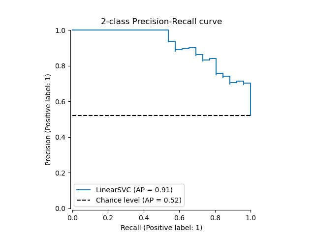
Let’s first plot the precision-recall curve without the classifier predictions. We use from_estimator that computes the predictions for us before plotting the curve.

from sklearn.metrics import PrecisionRecallDisplay

display = PrecisionRecallDisplay.from_estimator(
    classifier, X_test, y_test, name="LinearSVC", plot_chance_level=True, despine=True
)
_ = display.ax_.set_title("2-class Precision-Recall curve")

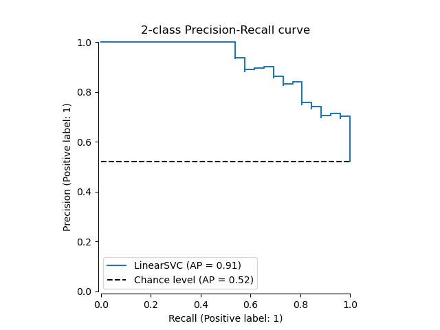
If we already got the estimated probabilities or scores for our model, then we can use from_predictions.

y_score = classifier.decision_function(X_test)

display = PrecisionRecallDisplay.from_predictions(
    y_test, y_score, name="LinearSVC", plot_chance_level=True, despine=True
)
_ = display.ax_.set_title("2-class Precision-Recall curve")

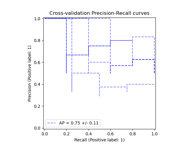
The from_cv_results takes the cross-validation results from cross_validate and plots a precision-recall curve for each fold.

from sklearn.model_selection import cross_validate

classifier = make_pipeline(StandardScaler(), LinearSVC(random_state=random_state))
cv_results = cross_validate(
    classifier, X_train, y_train, return_estimator=True, return_indices=True
)
display = PrecisionRecallDisplay.from_cv_results(cv_results, X_train, y_train)
_ = display.ax_.set_title("Cross-validation Precision-Recall curves")

In multi-label settings

The precision-recall curve does not support the multilabel setting. However, one can decide how to handle this case. We show such an example below.

Create multi-label data, fit, and predict

We create a multi-label dataset, to illustrate the precision-recall in multi-label settings.

from sklearn.preprocessing import label_binarize

# Use label_binarize to be multi-label like settings
Y = label_binarize(y, classes=[0, 1, 2])
n_classes = Y.shape[1]

# Split into training and test
X_train, X_test, Y_train, Y_test = train_test_split(
    X, Y, test_size=0.5, random_state=random_state
)

We use OneVsRestClassifier for multi-label prediction.

from sklearn.multiclass import OneVsRestClassifier

classifier = OneVsRestClassifier(
    make_pipeline(StandardScaler(), LinearSVC(random_state=random_state))
)
classifier.fit(X_train, Y_train)
y_score = classifier.decision_function(X_test)

The average precision score in multi-label settings

from sklearn.metrics import average_precision_score, precision_recall_curve

# For each class
precision = dict()
recall = dict()
average_precision = dict()
for i in range(n_classes):
    precision[i], recall[i], _ = precision_recall_curve(Y_test[:, i], y_score[:, i])
    average_precision[i] = average_precision_score(Y_test[:, i], y_score[:, i])

# A "micro-average": quantifying score on all classes jointly
precision["micro"], recall["micro"], _ = precision_recall_curve(
    Y_test.ravel(), y_score.ravel()
)
average_precision["micro"] = average_precision_score(Y_test, y_score, average="micro")

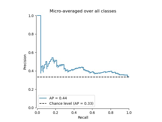
Plot the micro-averaged Precision-Recall curve

from collections import Counter

display = PrecisionRecallDisplay(
    recall=recall["micro"],
    precision=precision["micro"],
    average_precision=average_precision["micro"],
    prevalence_pos_label=Counter(Y_test.ravel())[1] / Y_test.size,
)
display.plot(plot_chance_level=True, despine=True)
_ = display.ax_.set_title("Micro-averaged over all classes")

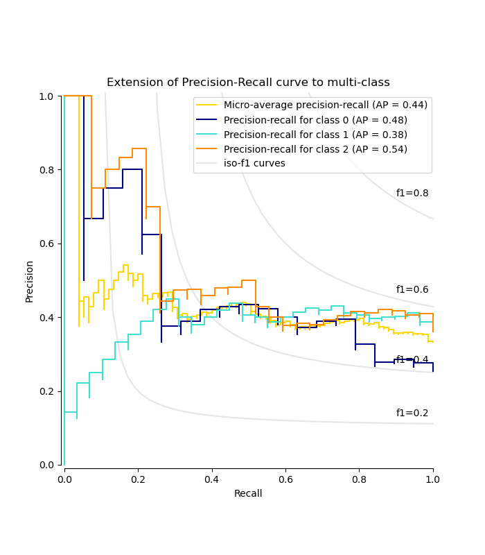
Plot Precision-Recall curve for each class and iso-f1 curves

from itertools import cycle

import matplotlib.pyplot as plt

# setup plot details
colors = cycle(["navy", "turquoise", "darkorange", "cornflowerblue", "teal"])

_, ax = plt.subplots(figsize=(7, 8))

f_scores = np.linspace(0.2, 0.8, num=4)
lines, labels = [], []
for f_score in f_scores:
    x = np.linspace(0.01, 1)
    y = f_score * x / (2 * x - f_score)
    (l,) = plt.plot(x[y >= 0], y[y >= 0], color="gray", alpha=0.2)
    plt.annotate("f1={0:0.1f}".format(f_score), xy=(0.9, y[45] + 0.02))

display = PrecisionRecallDisplay(
    recall=recall["micro"],
    precision=precision["micro"],
    average_precision=average_precision["micro"],
)
display.plot(
    ax=ax, name="Micro-average precision-recall", curve_kwargs={"color": "gold"}
)

for i, color in zip(range(n_classes), colors):
    display = PrecisionRecallDisplay(
        recall=recall[i],
        precision=precision[i],
        average_precision=average_precision[i],
    )
    display.plot(
        ax=ax,
        name=f"Precision-recall for class {i}",
        curve_kwargs={"color": color},
        despine=True,
    )

# add the legend for the iso-f1 curves
handles, labels = display.ax_.get_legend_handles_labels()
handles.extend([l])
labels.extend(["iso-f1 curves"])
# set the legend and the axes
ax.legend(handles=handles, labels=labels, loc="best")
ax.set_title("Extension of Precision-Recall curve to multi-class")

plt.show()

Related examples

Custom refit strategy of a grid search with cross-validation

Custom refit strategy of a grid search with cross-validation

Visualizations with Display Objects

Visualizations with Display Objects

Sparse inverse covariance estimation

Sparse inverse covariance estimation

Post-tuning the decision threshold for cost-sensitive learning

Post-tuning the decision threshold for cost-sensitive learning