Note
Go to the end to download the full example code or to run this example in your browser via JupyterLite or Binder.
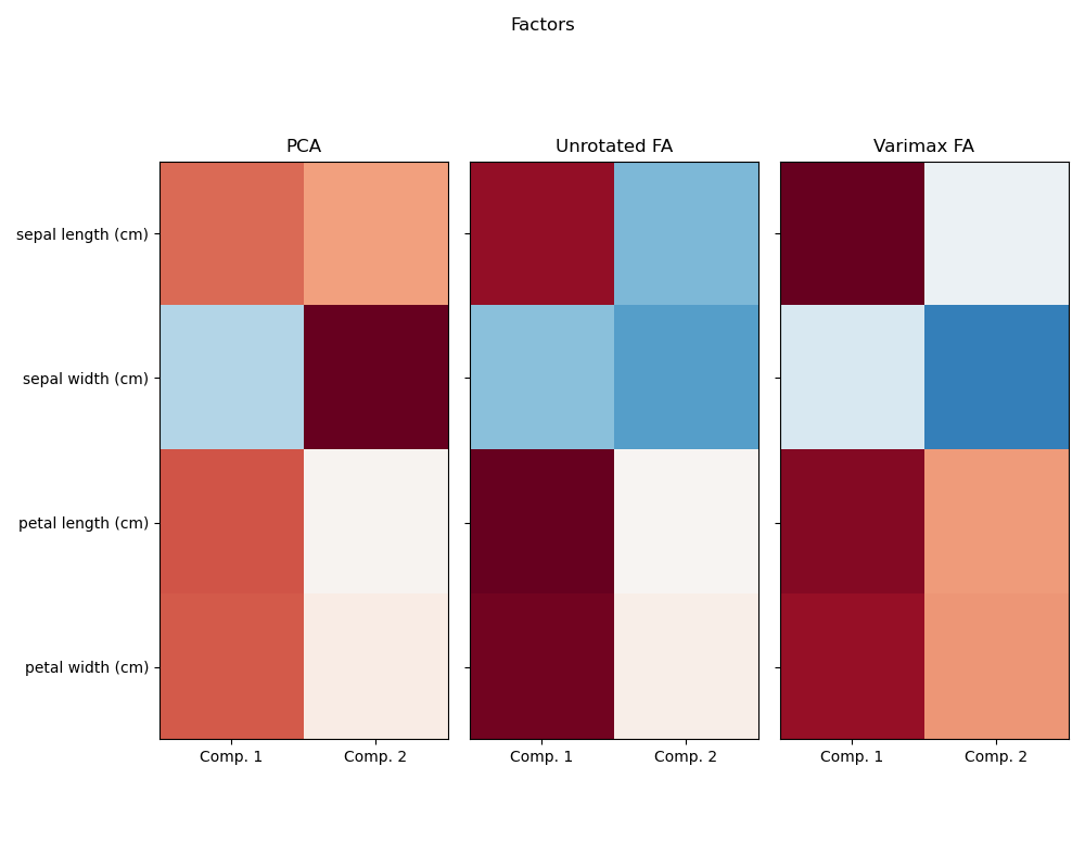
Factor Analysis (with rotation) to visualize patterns#
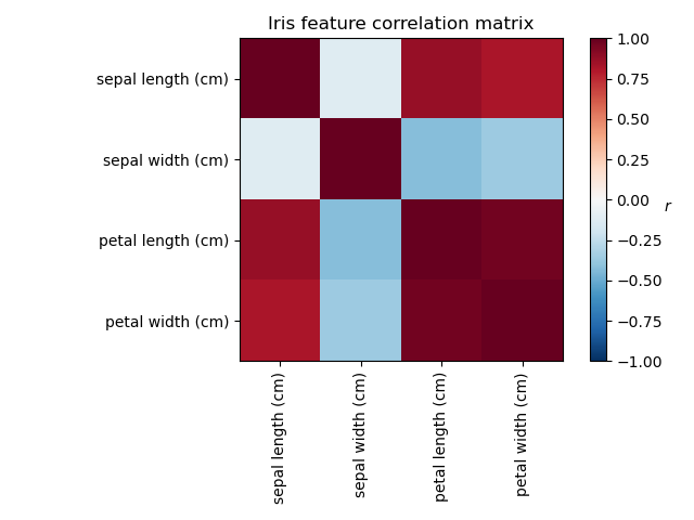
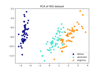
Investigating the Iris dataset, we see that sepal length, petal length and petal width are highly correlated. Sepal width is less redundant. Matrix decomposition techniques can uncover these latent patterns. Applying rotations to the resulting components does not inherently improve the predictive value of the derived latent space, but can help visualise their structure; here, for example, the varimax rotation, which is found by maximizing the squared variances of the weights, finds a structure where the second component only loads positively on sepal width.
# Authors: The scikit-learn developers
# SPDX-License-Identifier: BSD-3-Clause

import matplotlib.pyplot as plt
import numpy as np

from sklearn.datasets import load_iris
from sklearn.decomposition import PCA, FactorAnalysis
from sklearn.preprocessing import StandardScaler
Load Iris data
data = load_iris()
X = StandardScaler().fit_transform(data["data"])
feature_names = data["feature_names"]
Plot covariance of Iris features
ax = plt.axes()

im = ax.imshow(np.corrcoef(X.T), cmap="RdBu_r", vmin=-1, vmax=1)

ax.set_xticks([0, 1, 2, 3])
ax.set_xticklabels(list(feature_names), rotation=90)
ax.set_yticks([0, 1, 2, 3])
ax.set_yticklabels(list(feature_names))

plt.colorbar(im).ax.set_ylabel("$r$", rotation=0)
ax.set_title("Iris feature correlation matrix")
plt.tight_layout()
Run factor analysis with Varimax rotation
n_comps = 2

methods = [
    ("PCA", PCA()),
    ("Unrotated FA", FactorAnalysis()),
    ("Varimax FA", FactorAnalysis(rotation="varimax")),
]
fig, axes = plt.subplots(ncols=len(methods), figsize=(10, 8), sharey=True)

for ax, (method, fa) in zip(axes, methods):
    fa.set_params(n_components=n_comps)
    fa.fit(X)

    components = fa.components_.T
    print("\n\n %s :\n" % method)
    print(components)

    vmax = np.abs(components).max()
    ax.imshow(components, cmap="RdBu_r", vmax=vmax, vmin=-vmax)
    ax.set_yticks(np.arange(len(feature_names)))
    ax.set_yticklabels(feature_names)
    ax.set_title(str(method))
    ax.set_xticks([0, 1])
    ax.set_xticklabels(["Comp. 1", "Comp. 2"])
fig.suptitle("Factors")
plt.tight_layout()
plt.show()
 PCA :

[[ 0.52106591  0.37741762]
 [-0.26934744  0.92329566]
 [ 0.5804131   0.02449161]
 [ 0.56485654  0.06694199]]


 Unrotated FA :

[[ 0.88096009 -0.4472869 ]
 [-0.41691605 -0.55390036]
 [ 0.99918858  0.01915283]
 [ 0.96228895  0.05840206]]


 Varimax FA :

[[ 0.98633022 -0.05752333]
 [-0.16052385 -0.67443065]
 [ 0.90809432  0.41726413]
 [ 0.85857475  0.43847489]]
Total running time of the script: (0 minutes 0.383 seconds)
Related examples
Principal Component Analysis (PCA) on Iris Dataset
Comparison of LDA and PCA 2D projection of Iris dataset
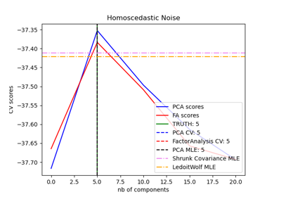
Model selection with Probabilistic PCA and Factor Analysis (FA)