Note
Go to the end to download the full example code or to run this example in your browser via JupyterLite or Binder.
Decision Tree Regression#
In this example, we demonstrate the effect of changing the maximum depth of a decision tree on how it fits to the data. We perform this once on a 1D regression task and once on a multi-output regression task.
# Authors: The scikit-learn developers
# SPDX-License-Identifier: BSD-3-Clause
Decision Tree on a 1D Regression Task#
Here we fit a tree on a 1D regression task.
The decision trees is used to fit a sine curve with addition noisy observation. As a result, it learns local linear regressions approximating the sine curve.
We can see that if the maximum depth of the tree (controlled by the
max_depth parameter) is set too high, the decision trees learn too fine
details of the training data and learn from the noise, i.e. they overfit.
Create a random 1D dataset#
import numpy as np

rng = np.random.RandomState(1)
X = np.sort(5 * rng.rand(80, 1), axis=0)
y = np.sin(X).ravel()
y[::5] += 3 * (0.5 - rng.rand(16))
Fit regression model#
Here we fit two models with different maximum depths
from sklearn.tree import DecisionTreeRegressor

regr_1 = DecisionTreeRegressor(max_depth=2)
regr_2 = DecisionTreeRegressor(max_depth=5)
regr_1.fit(X, y)
regr_2.fit(X, y)
Predict#
Get predictions on the test set
X_test = np.arange(0.0, 5.0, 0.01)[:, np.newaxis]
y_1 = regr_1.predict(X_test)
y_2 = regr_2.predict(X_test)
Plot the results#
import matplotlib.pyplot as plt

plt.figure()
plt.scatter(X, y, s=20, edgecolor="black", c="darkorange", label="data")
plt.plot(X_test, y_1, color="cornflowerblue", label="max_depth=2", linewidth=2)
plt.plot(X_test, y_2, color="yellowgreen", label="max_depth=5", linewidth=2)
plt.xlabel("data")
plt.ylabel("target")
plt.title("Decision Tree Regression")
plt.legend()
plt.show()
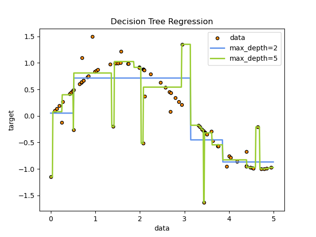
As you can see, the model with a depth of 5 (yellow) learns the details of the training data to the point that it overfits to the noise. On the other hand, the model with a depth of 2 (blue) learns the major tendencies in the data well and does not overfit. In real use cases, you need to make sure that the tree is not overfitting the training data, which can be done using cross-validation.
Decision Tree Regression with Multi-Output Targets#
Here the decision trees
is used to predict simultaneously the noisy x and y observations of a circle
given a single underlying feature. As a result, it learns local linear
regressions approximating the circle.
We can see that if the maximum depth of the tree (controlled by the
max_depth parameter) is set too high, the decision trees learn too fine
details of the training data and learn from the noise, i.e. they overfit.
Create a random dataset#
Fit regression model#
regr_1 = DecisionTreeRegressor(max_depth=2)
regr_2 = DecisionTreeRegressor(max_depth=5)
regr_3 = DecisionTreeRegressor(max_depth=8)
regr_1.fit(X, y)
regr_2.fit(X, y)
regr_3.fit(X, y)
Predict#
Get predictions on the test set
X_test = np.arange(-100.0, 100.0, 0.01)[:, np.newaxis]
y_1 = regr_1.predict(X_test)
y_2 = regr_2.predict(X_test)
y_3 = regr_3.predict(X_test)
Plot the results#
plt.figure()
s = 25
plt.scatter(y[:, 0], y[:, 1], c="yellow", s=s, edgecolor="black", label="data")
plt.scatter(
    y_1[:, 0],
    y_1[:, 1],
    c="cornflowerblue",
    s=s,
    edgecolor="black",
    label="max_depth=2",
)
plt.scatter(y_2[:, 0], y_2[:, 1], c="red", s=s, edgecolor="black", label="max_depth=5")
plt.scatter(y_3[:, 0], y_3[:, 1], c="blue", s=s, edgecolor="black", label="max_depth=8")
plt.xlim([-6, 6])
plt.ylim([-6, 6])
plt.xlabel("target 1")
plt.ylabel("target 2")
plt.title("Multi-output Decision Tree Regression")
plt.legend(loc="best")
plt.show()
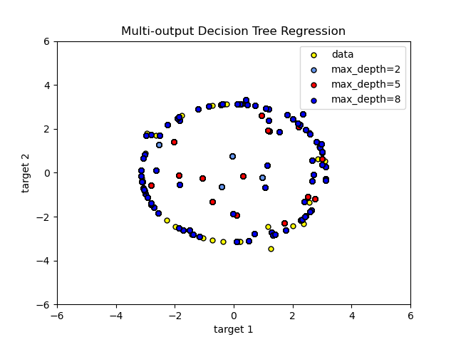
As you can see, the higher the value of max_depth, the more details of the data
are caught by the model. However, the model also overfits to the data and is
influenced by the noise.
Total running time of the script: (0 minutes 0.400 seconds)
Related examples
Comparing random forests and the multi-output meta estimator
Plot the decision surfaces of ensembles of trees on the iris dataset
