Note

Go to the end to download the full example code or to run this example in your browser via JupyterLite or Binder

Demo of OPTICS clustering algorithm¶

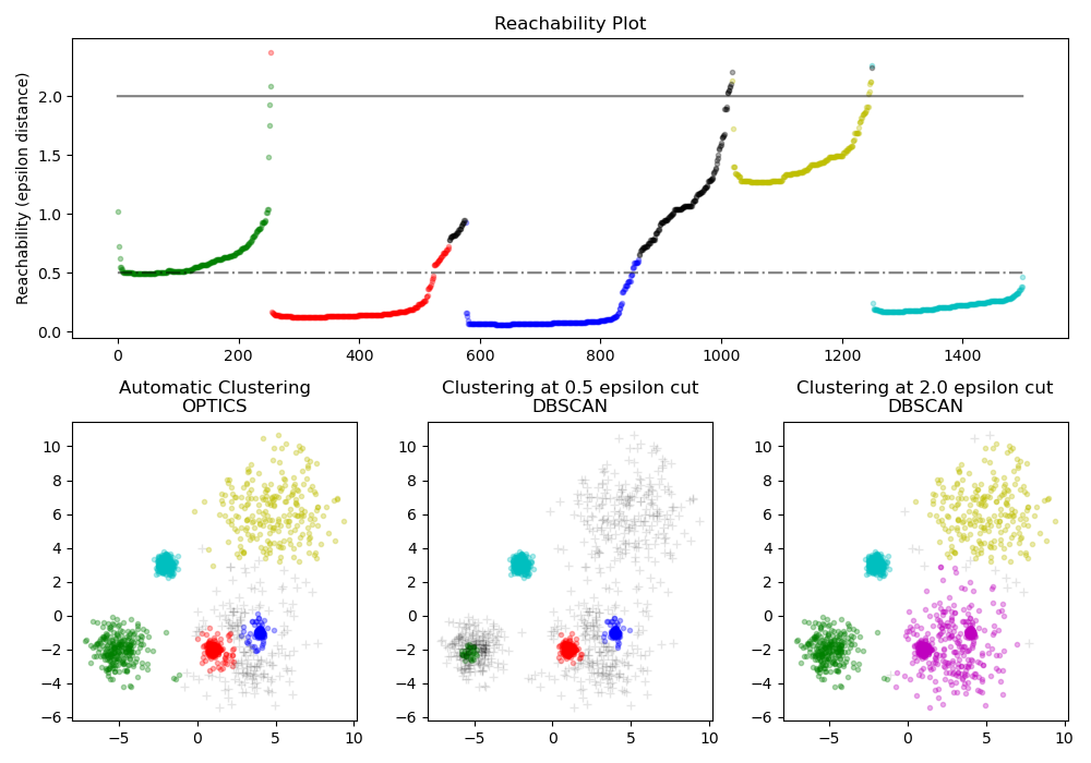
Finds core samples of high density and expands clusters from them. This example uses data that is generated so that the clusters have different densities.

The OPTICS is first used with its Xi cluster detection method, and then setting specific thresholds on the reachability, which corresponds to DBSCAN. We can see that the different clusters of OPTICS’s Xi method can be recovered with different choices of thresholds in DBSCAN.

Reachability Plot, Automatic Clustering OPTICS, Clustering at 0.5 epsilon cut DBSCAN, Clustering at 2.0 epsilon cut DBSCAN

# Authors: Shane Grigsby <refuge@rocktalus.com>
#          Adrin Jalali <adrin.jalali@gmail.com>
# License: BSD 3 clause

import matplotlib.gridspec as gridspec
import matplotlib.pyplot as plt
import numpy as np

from sklearn.cluster import OPTICS, cluster_optics_dbscan

# Generate sample data

np.random.seed(0)
n_points_per_cluster = 250

C1 = [-5, -2] + 0.8 * np.random.randn(n_points_per_cluster, 2)
C2 = [4, -1] + 0.1 * np.random.randn(n_points_per_cluster, 2)
C3 = [1, -2] + 0.2 * np.random.randn(n_points_per_cluster, 2)
C4 = [-2, 3] + 0.3 * np.random.randn(n_points_per_cluster, 2)
C5 = [3, -2] + 1.6 * np.random.randn(n_points_per_cluster, 2)
C6 = [5, 6] + 2 * np.random.randn(n_points_per_cluster, 2)
X = np.vstack((C1, C2, C3, C4, C5, C6))

clust = OPTICS(min_samples=50, xi=0.05, min_cluster_size=0.05)

# Run the fit
clust.fit(X)

labels_050 = cluster_optics_dbscan(
    reachability=clust.reachability_,
    core_distances=clust.core_distances_,
    ordering=clust.ordering_,
    eps=0.5,
)
labels_200 = cluster_optics_dbscan(
    reachability=clust.reachability_,
    core_distances=clust.core_distances_,
    ordering=clust.ordering_,
    eps=2,
)

space = np.arange(len(X))
reachability = clust.reachability_[clust.ordering_]
labels = clust.labels_[clust.ordering_]

plt.figure(figsize=(10, 7))
G = gridspec.GridSpec(2, 3)
ax1 = plt.subplot(G[0, :])
ax2 = plt.subplot(G[1, 0])
ax3 = plt.subplot(G[1, 1])
ax4 = plt.subplot(G[1, 2])

# Reachability plot
colors = ["g.", "r.", "b.", "y.", "c."]
for klass, color in enumerate(colors):
    Xk = space[labels == klass]
    Rk = reachability[labels == klass]
    ax1.plot(Xk, Rk, color, alpha=0.3)
ax1.plot(space[labels == -1], reachability[labels == -1], "k.", alpha=0.3)
ax1.plot(space, np.full_like(space, 2.0, dtype=float), "k-", alpha=0.5)
ax1.plot(space, np.full_like(space, 0.5, dtype=float), "k-.", alpha=0.5)
ax1.set_ylabel("Reachability (epsilon distance)")
ax1.set_title("Reachability Plot")

# OPTICS
colors = ["g.", "r.", "b.", "y.", "c."]
for klass, color in enumerate(colors):
    Xk = X[clust.labels_ == klass]
    ax2.plot(Xk[:, 0], Xk[:, 1], color, alpha=0.3)
ax2.plot(X[clust.labels_ == -1, 0], X[clust.labels_ == -1, 1], "k+", alpha=0.1)
ax2.set_title("Automatic Clustering\nOPTICS")

# DBSCAN at 0.5
colors = ["g.", "r.", "b.", "c."]
for klass, color in enumerate(colors):
    Xk = X[labels_050 == klass]
    ax3.plot(Xk[:, 0], Xk[:, 1], color, alpha=0.3)
ax3.plot(X[labels_050 == -1, 0], X[labels_050 == -1, 1], "k+", alpha=0.1)
ax3.set_title("Clustering at 0.5 epsilon cut\nDBSCAN")

# DBSCAN at 2.
colors = ["g.", "m.", "y.", "c."]
for klass, color in enumerate(colors):
    Xk = X[labels_200 == klass]
    ax4.plot(Xk[:, 0], Xk[:, 1], color, alpha=0.3)
ax4.plot(X[labels_200 == -1, 0], X[labels_200 == -1, 1], "k+", alpha=0.1)
ax4.set_title("Clustering at 2.0 epsilon cut\nDBSCAN")

plt.tight_layout()
plt.show()