Note
Go to the end to download the full example code or to run this example in your browser via JupyterLite or Binder.
Release Highlights for scikit-learn 1.8#
We are pleased to announce the release of scikit-learn 1.8! Many bug fixes and improvements were added, as well as some key new features. Below we detail the highlights of this release. For an exhaustive list of all the changes, please refer to the release notes.
To install the latest version (with pip):
pip install --upgrade scikit-learn
or with conda:
conda install -c conda-forge scikit-learn
Array API support (enables GPU computations)#
The progressive adoption of the Python array API standard in scikit-learn means that PyTorch and CuPy input arrays are used directly. This means that in scikit-learn estimators and functions non-CPU devices, such as GPUs, can be used to perform the computation. As a result performance is improved and integration with these libraries is easier.
In scikit-learn 1.8, several estimators and functions have been updated to support array API compatible inputs, for example PyTorch tensors and CuPy arrays.
Array API support was added to the following estimators:
preprocessing.StandardScaler,
preprocessing.PolynomialFeatures, linear_model.RidgeCV,
linear_model.RidgeClassifierCV, mixture.GaussianMixture and
calibration.CalibratedClassifierCV.
Array API support was also added to several metrics in sklearn.metrics
module, see Support for array API compatible inputs for more details.
Please refer to the array API support page for instructions to use scikit-learn with array API compatible libraries such as PyTorch or CuPy. Note: Array API support is experimental and must be explicitly enabled both in SciPy and scikit-learn.
Here is an excerpt of using a feature engineering preprocessor on the CPU,
followed by calibration.CalibratedClassifierCV
and linear_model.RidgeCV together on a GPU with the help of PyTorch:
ridge_pipeline_gpu = make_pipeline(
    # Ensure that all features (including categorical features) are preprocessed
    # on the CPU and mapped to a numerical representation.
    feature_preprocessor,
    # Move the results to the GPU and perform computations there
    FunctionTransformer(
        lambda x: torch.tensor(x.to_numpy().astype(np.float32), device="cuda"))
    ,
    CalibratedClassifierCV(
        RidgeClassifierCV(alphas=alphas), method="temperature"
    ),
)
with sklearn.config_context(array_api_dispatch=True):
    cv_results = cross_validate(ridge_pipeline_gpu, features, target)
See the full notebook on Google Colab for more details. On this particular example, using the Colab GPU vs using a single CPU core leads to a 10x speedup which is quite typical for such workloads.
Free-threaded CPython 3.14 support#
scikit-learn has support for free-threaded CPython, in particular free-threaded wheels are available for all of our supported platforms on Python 3.14.
We would be very interested by user feedback. Here are a few things you can try:
install free-threaded CPython 3.14, run your favourite scikit-learn script and check that nothing breaks unexpectedly. Note that CPython 3.14 (rather than 3.13) is strongly advised because a number of free-threaded bugs have been fixed since CPython 3.13.
if you use some estimators with a
n_jobsparameter, try changing the default backend to threading withjoblib.parallel_configas in the snippet below. This could potentially speed-up your code because the default joblib backend is process-based and incurs more overhead than threads.grid_search = GridSearchCV(clf, param_grid=param_grid, n_jobs=4) with joblib.parallel_config(backend="threading"): grid_search.fit(X, y)
don’t hesitate to report any issue or unexpected performance behaviour by opening a GitHub issue!
Free-threaded (also known as nogil) CPython is a version of CPython that aims to enable efficient multi-threaded use cases by removing the Global Interpreter Lock (GIL).
For more details about free-threaded CPython see py-free-threading doc, in particular how to install a free-threaded CPython and Ecosystem compatibility tracking.
In scikit-learn, one hope with free-threaded Python is to more efficiently
leverage multi-core CPUs by using thread workers instead of subprocess
workers for parallel computation when passing n_jobs>1 in functions or
estimators. Efficiency gains are expected by removing the need for
inter-process communication. Be aware that switching the default joblib
backend and testing that everything works well with free-threaded Python is an
ongoing long-term effort.
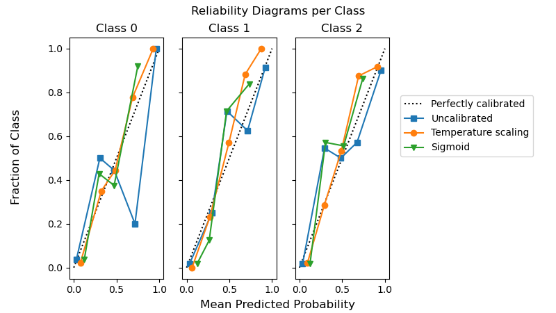
Temperature scaling in CalibratedClassifierCV#
Probability calibration of classifiers with temperature scaling is available in
calibration.CalibratedClassifierCV by setting method="temperature".
This method is particularly well suited for multiclass problems because it provides
(better) calibrated probabilities with a single free parameter. This is in
contrast to all the other available calibrations methods
which use a “One-vs-Rest” scheme that adds more parameters for each class.
from sklearn.calibration import CalibratedClassifierCV
from sklearn.datasets import make_classification
from sklearn.naive_bayes import GaussianNB

X, y = make_classification(n_classes=3, n_informative=8, random_state=42)
clf = GaussianNB().fit(X, y)
sig = CalibratedClassifierCV(clf, method="sigmoid", ensemble=False).fit(X, y)
ts = CalibratedClassifierCV(clf, method="temperature", ensemble=False).fit(X, y)
The following example shows that temperature scaling can produce better calibrated probabilities than sigmoid calibration in multi-class classification problem with 3 classes.
import matplotlib.pyplot as plt

from sklearn.calibration import CalibrationDisplay

fig, axes = plt.subplots(
    figsize=(8, 4.5),
    ncols=3,
    sharey=True,
)
for i, c in enumerate(ts.classes_):
    CalibrationDisplay.from_predictions(
        y == c, clf.predict_proba(X)[:, i], name="Uncalibrated", ax=axes[i], marker="s"
    )
    CalibrationDisplay.from_predictions(
        y == c,
        ts.predict_proba(X)[:, i],
        name="Temperature scaling",
        ax=axes[i],
        marker="o",
    )
    CalibrationDisplay.from_predictions(
        y == c, sig.predict_proba(X)[:, i], name="Sigmoid", ax=axes[i], marker="v"
    )
    axes[i].set_title(f"Class {c}")
    axes[i].set_xlabel(None)
    axes[i].set_ylabel(None)
    axes[i].get_legend().remove()
fig.suptitle("Reliability Diagrams per Class")
fig.supxlabel("Mean Predicted Probability")
fig.supylabel("Fraction of Class")
fig.legend(*axes[0].get_legend_handles_labels(), loc=(0.72, 0.5))
plt.subplots_adjust(right=0.7)
_ = fig.show()
Efficiency improvements in linear models#
The fit time has been massively reduced for squared error based estimators
with L1 penalty: ElasticNet, Lasso, MultiTaskElasticNet,
MultiTaskLasso and their CV variants. The fit time improvement is mainly
achieved by gap safe screening rules. They enable the coordinate descent
solver to set feature coefficients to zero early on and not look at them
again. The stronger the L1 penalty the earlier features can be excluded from
further updates.
from time import time

from sklearn.datasets import make_regression
from sklearn.linear_model import ElasticNetCV

X, y = make_regression(n_features=10_000, random_state=0)
model = ElasticNetCV()
tic = time()
model.fit(X, y)
toc = time()
print(f"Fitting ElasticNetCV took {toc - tic:.3} seconds.")
Fitting ElasticNetCV took 17.4 seconds.
HTML representation of estimators#
Hyperparameters in the dropdown table of the HTML representation now include links to the online documentation. Docstring descriptions are also shown as tooltips on hover.
from sklearn.linear_model import LogisticRegression
from sklearn.pipeline import make_pipeline
from sklearn.preprocessing import StandardScaler

clf = make_pipeline(StandardScaler(), LogisticRegression(C=10))
Expand the estimator diagram below by clicking on “LogisticRegression” and then on “Parameters”.
clf
DecisionTreeRegressor with criterion="absolute_error"#
tree.DecisionTreeRegressor with criterion="absolute_error"
now runs much faster. It has now O(n * log(n)) complexity compared to
O(n**2) previously, which allows to scale to millions of data points.
As an illustration, on a dataset with 100_000 samples and 1 feature, doing a single split takes of the order of 100 ms, compared to ~20 seconds before.
import time

from sklearn.datasets import make_regression
from sklearn.tree import DecisionTreeRegressor

X, y = make_regression(n_samples=100_000, n_features=1)
tree = DecisionTreeRegressor(criterion="absolute_error", max_depth=1)

tic = time.time()
tree.fit(X, y)
elapsed = time.time() - tic
print(f"Fit took {elapsed:.2f} seconds")
Fit took 0.16 seconds
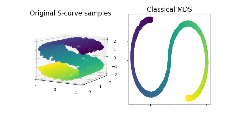
ClassicalMDS#
Classical MDS, also known as “Principal Coordinates Analysis” (PCoA)
or “Torgerson’s scaling” is now available within the sklearn.manifold
module. Classical MDS is close to PCA and instead of approximating
distances, it approximates pairwise scalar products, which has an exact
analytic solution in terms of eigendecomposition.
Let’s illustrate this new addition by using it on an S-curve dataset to get a low-dimensional representation of the data.
import matplotlib.pyplot as plt
from matplotlib import ticker

from sklearn import datasets, manifold

n_samples = 1500
S_points, S_color = datasets.make_s_curve(n_samples, random_state=0)
md_classical = manifold.ClassicalMDS(n_components=2)
S_scaling = md_classical.fit_transform(S_points)

fig = plt.figure(figsize=(8, 4))
ax1 = fig.add_subplot(1, 2, 1, projection="3d")
x, y, z = S_points.T
ax1.scatter(x, y, z, c=S_color, s=50, alpha=0.8)
ax1.set_title("Original S-curve samples", size=16)
ax1.view_init(azim=-60, elev=9)
for axis in (ax1.xaxis, ax1.yaxis, ax1.zaxis):
    axis.set_major_locator(ticker.MultipleLocator(1))

ax2 = fig.add_subplot(1, 2, 2)
x2, y2 = S_scaling.T
ax2.scatter(x2, y2, c=S_color, s=50, alpha=0.8)
ax2.set_title("Classical MDS", size=16)
for axis in (ax2.xaxis, ax2.yaxis):
    axis.set_major_formatter(ticker.NullFormatter())

plt.show()
Total running time of the script: (0 minutes 18.474 seconds)
Related examples