Note

Go to the end to download the full example code. or to run this example in your browser via JupyterLite or Binder

Ridge coefficients as a function of the L2 Regularization#

A model that overfits learns the training data too well, capturing both the underlying patterns and the noise in the data. However, when applied to unseen data, the learned associations may not hold. We normally detect this when we apply our trained predictions to the test data and see the statistical performance drop significantly compared to the training data.

One way to overcome overfitting is through regularization, which can be done by penalizing large weights (coefficients) in linear models, forcing the model to shrink all coefficients. Regularization reduces a model’s reliance on specific information obtained from the training samples.

This example illustrates how L2 regularization in a Ridge regression affects a model’s performance by adding a penalty term to the loss that increases with the coefficients \(\beta\).

The regularized loss function is given by: \(\mathcal{L}(X, y, \beta) = \| y - X \beta \|^{2}_{2} + \alpha \| \beta \|^{2}_{2}\)

where \(X\) is the input data, \(y\) is the target variable, \(\beta\) is the vector of coefficients associated with the features, and \(\alpha\) is the regularization strength.

The regularized loss function aims to balance the trade-off between accurately predicting the training set and to prevent overfitting.

In this regularized loss, the left-hand side (e.g. \(\|y - X\beta\|^{2}_{2}\)) measures the squared difference between the actual target variable, \(y\), and the predicted values. Minimizing this term alone could lead to overfitting, as the model may become too complex and sensitive to noise in the training data.

To address overfitting, Ridge regularization adds a constraint, called a penalty term, (\(\alpha \| \beta\|^{2}_{2}\)) to the loss function. This penalty term is the sum of the squares of the model’s coefficients, multiplied by the regularization strength \(\alpha\). By introducing this constraint, Ridge regularization discourages any single coefficient \(\beta_{i}\) from taking an excessively large value and encourages smaller and more evenly distributed coefficients. Higher values of \(\alpha\) force the coefficients towards zero. However, an excessively high \(\alpha\) can result in an underfit model that fails to capture important patterns in the data.

Therefore, the regularized loss function combines the prediction accuracy term and the penalty term. By adjusting the regularization strength, practitioners can fine-tune the degree of constraint imposed on the weights, training a model capable of generalizing well to unseen data while avoiding overfitting.

# Authors: The scikit-learn developers
# SPDX-License-Identifier: BSD-3-Clause

Purpose of this example#

For the purpose of showing how Ridge regularization works, we will create a non-noisy data set. Then we will train a regularized model on a range of regularization strengths (\(\alpha\)) and plot how the trained coefficients and the mean squared error between those and the original values behave as functions of the regularization strength.

Creating a non-noisy data set#

We make a toy data set with 100 samples and 10 features, that’s suitable to detect regression. Out of the 10 features, 8 are informative and contribute to the regression, while the remaining 2 features do not have any effect on the target variable (their true coefficients are 0). Please note that in this example the data is non-noisy, hence we can expect our regression model to recover exactly the true coefficients w.

from sklearn.datasets import make_regression

X, y, w = make_regression(
    n_samples=100, n_features=10, n_informative=8, coef=True, random_state=1
)

# Obtain the true coefficients
print(f"The true coefficient of this regression problem are:\n{w}")

The true coefficient of this regression problem are:
[38.32634568 88.49665188  0.         29.75747153  0.         19.08699432
 25.44381023 38.69892343 49.28808734 71.75949622]

Training the Ridge Regressor#

We use Ridge, a linear model with L2 regularization. We train several models, each with a different value for the model parameter alpha, which is a positive constant that multiplies the penalty term, controlling the regularization strength. For each trained model we then compute the error between the true coefficients w and the coefficients found by the model clf. We store the identified coefficients and the calculated errors for the corresponding coefficients in lists, which makes it convenient for us to plot them.

import numpy as np

from sklearn.linear_model import Ridge
from sklearn.metrics import mean_squared_error

clf = Ridge()

# Generate values for `alpha` that are evenly distributed on a logarithmic scale
alphas = np.logspace(-3, 4, 200)
coefs = []
errors_coefs = []

# Train the model with different regularisation strengths
for a in alphas:
    clf.set_params(alpha=a).fit(X, y)
    coefs.append(clf.coef_)
    errors_coefs.append(mean_squared_error(clf.coef_, w))

Plotting trained Coefficients and Mean Squared Errors#

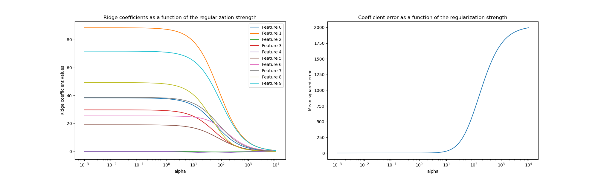
We now plot the 10 different regularized coefficients as a function of the regularization parameter alpha where each color represents a different coefficient.

On the right-hand-side, we plot how the errors of the coefficients from the estimator change as a function of regularization.

import matplotlib.pyplot as plt
import pandas as pd

alphas = pd.Index(alphas, name="alpha")
coefs = pd.DataFrame(coefs, index=alphas, columns=[f"Feature {i}" for i in range(10)])
errors = pd.Series(errors_coefs, index=alphas, name="Mean squared error")

fig, axs = plt.subplots(1, 2, figsize=(20, 6))

coefs.plot(
    ax=axs[0],
    logx=True,
    title="Ridge coefficients as a function of the regularization strength",
)
axs[0].set_ylabel("Ridge coefficient values")
errors.plot(
    ax=axs[1],
    logx=True,
    title="Coefficient error as a function of the regularization strength",
)
_ = axs[1].set_ylabel("Mean squared error")

Ridge coefficients as a function of the regularization strength, Coefficient error as a function of the regularization strength

Interpreting the plots#

The plot on the left-hand side shows how the regularization strength (alpha) affects the Ridge regression coefficients. Smaller values of alpha (weak regularization), allow the coefficients to closely resemble the true coefficients (w) used to generate the data set. This is because no additional noise was added to our artificial data set. As alpha increases, the coefficients shrink towards zero, gradually reducing the impact of the features that were formerly more significant.

The right-hand side plot shows the mean squared error (MSE) between the coefficients found by the model and the true coefficients (w). It provides a measure that relates to how exact our ridge model is in comparison to the true generative model. A low error means that it found coefficients closer to the ones of the true generative model. In this case, since our toy data set was non-noisy, we can see that the least regularized model retrieves coefficients closest to the true coefficients (w) (error is close to 0).

When alpha is small, the model captures the intricate details of the training data, whether those were caused by noise or by actual information. As alpha increases, the highest coefficients shrink more rapidly, rendering their corresponding features less influential in the training process. This can enhance a model’s ability to generalize to unseen data (if there was a lot of noise to capture), but it also poses the risk of losing performance if the regularization becomes too strong compared to the amount of noise the data contained (as in this example).

In real-world scenarios where data typically includes noise, selecting an appropriate alpha value becomes crucial in striking a balance between an overfitting and an underfitting model.

Here, we saw that Ridge adds a penalty to the coefficients to fight overfitting. Another problem that occurs is linked to the presence of outliers in the training dataset. An outlier is a data point that differs significantly from other observations. Concretely, these outliers impact the left-hand side term of the loss function that we showed earlier. Some other linear models are formulated to be robust to outliers such as the HuberRegressor. You can learn more about it in the HuberRegressor vs Ridge on dataset with strong outliers example.

Total running time of the script: (0 minutes 0.713 seconds)