Note
Go to the end to download the full example code or to run this example in your browser via JupyterLite or Binder.
Comparing Target Encoder with Other Encoders#
The TargetEncoder uses the value of the target to encode each
categorical feature. In this example, we will compare three different approaches
for handling categorical features: TargetEncoder,
OrdinalEncoder, OneHotEncoder and dropping the category.
Note
fit(X, y).transform(X) does not equal fit_transform(X, y) because a
cross fitting scheme is used in fit_transform for encoding. See the
User Guide for details.
# Authors: The scikit-learn developers
# SPDX-License-Identifier: BSD-3-Clause
Loading Data from OpenML#
First, we load the wine reviews dataset, where the target is the points given be a reviewer:
from sklearn.datasets import fetch_openml

wine_reviews = fetch_openml(data_id=42074, as_frame=True)

df = wine_reviews.frame
df.head()
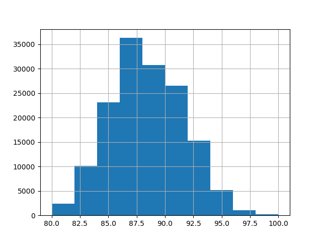
For this example, we use the following subset of numerical and categorical features in the data. The target are continuous values from 80 to 100:
numerical_features = ["price"]
categorical_features = [
    "country",
    "province",
    "region_1",
    "region_2",
    "variety",
    "winery",
]
target_name = "points"

X = df[numerical_features + categorical_features]
y = df[target_name]

_ = y.hist()
Training and Evaluating Pipelines with Different Encoders#
In this section, we will evaluate pipelines with
HistGradientBoostingRegressor with different encoding
strategies. First, we list out the encoders we will be using to preprocess
the categorical features:
from sklearn.compose import ColumnTransformer
from sklearn.preprocessing import OneHotEncoder, OrdinalEncoder, TargetEncoder

categorical_preprocessors = [
    ("drop", "drop"),
    ("ordinal", OrdinalEncoder(handle_unknown="use_encoded_value", unknown_value=-1)),
    (
        "one_hot",
        OneHotEncoder(handle_unknown="ignore", max_categories=20, sparse_output=False),
    ),
    ("target", TargetEncoder(target_type="continuous")),
]
Next, we evaluate the models using cross validation and record the results:
from sklearn.ensemble import HistGradientBoostingRegressor
from sklearn.model_selection import cross_validate
from sklearn.pipeline import make_pipeline

n_cv_folds = 3
max_iter = 20
results = []


def evaluate_model_and_store(name, pipe):
    result = cross_validate(
        pipe,
        X,
        y,
        scoring="neg_root_mean_squared_error",
        cv=n_cv_folds,
        return_train_score=True,
    )
    rmse_test_score = -result["test_score"]
    rmse_train_score = -result["train_score"]
    results.append(
        {
            "preprocessor": name,
            "rmse_test_mean": rmse_test_score.mean(),
            "rmse_test_std": rmse_train_score.std(),
            "rmse_train_mean": rmse_train_score.mean(),
            "rmse_train_std": rmse_train_score.std(),
        }
    )


for name, categorical_preprocessor in categorical_preprocessors:
    preprocessor = ColumnTransformer(
        [
            ("numerical", "passthrough", numerical_features),
            ("categorical", categorical_preprocessor, categorical_features),
        ]
    )
    pipe = make_pipeline(
        preprocessor, HistGradientBoostingRegressor(random_state=0, max_iter=max_iter)
    )
    evaluate_model_and_store(name, pipe)
Native Categorical Feature Support#
In this section, we build and evaluate a pipeline that uses native categorical
feature support in HistGradientBoostingRegressor,
which only supports up to 255 unique categories. In our dataset, the most of
the categorical features have more than 255 unique categories:
n_unique_categories = df[categorical_features].nunique().sort_values(ascending=False)
n_unique_categories
winery      14810
region_1     1236
variety       632
province      455
country        48
region_2       18
dtype: int64
To workaround the limitation above, we group the categorical features into low cardinality and high cardinality features. The high cardinality features will be target encoded and the low cardinality features will use the native categorical feature in gradient boosting.
high_cardinality_features = n_unique_categories[n_unique_categories > 255].index
low_cardinality_features = n_unique_categories[n_unique_categories <= 255].index
mixed_encoded_preprocessor = ColumnTransformer(
    [
        ("numerical", "passthrough", numerical_features),
        (
            "high_cardinality",
            TargetEncoder(target_type="continuous"),
            high_cardinality_features,
        ),
        (
            "low_cardinality",
            OrdinalEncoder(handle_unknown="use_encoded_value", unknown_value=-1),
            low_cardinality_features,
        ),
    ],
    verbose_feature_names_out=False,
)

# The output of the of the preprocessor must be set to pandas so the
# gradient boosting model can detect the low cardinality features.
mixed_encoded_preprocessor.set_output(transform="pandas")
mixed_pipe = make_pipeline(
    mixed_encoded_preprocessor,
    HistGradientBoostingRegressor(
        random_state=0, max_iter=max_iter, categorical_features=low_cardinality_features
    ),
)
mixed_pipe
Finally, we evaluate the pipeline using cross validation and record the results:
evaluate_model_and_store("mixed_target", mixed_pipe)
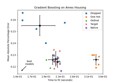
Plotting the Results#
In this section, we display the results by plotting the test and train scores:
import matplotlib.pyplot as plt
import pandas as pd

results_df = (
    pd.DataFrame(results).set_index("preprocessor").sort_values("rmse_test_mean")
)

fig, (ax1, ax2) = plt.subplots(
    1, 2, figsize=(12, 8), sharey=True, constrained_layout=True
)
xticks = range(len(results_df))
name_to_color = dict(
    zip((r["preprocessor"] for r in results), ["C0", "C1", "C2", "C3", "C4"])
)

for subset, ax in zip(["test", "train"], [ax1, ax2]):
    mean, std = f"rmse_{subset}_mean", f"rmse_{subset}_std"
    data = results_df[[mean, std]].sort_values(mean)
    ax.bar(
        x=xticks,
        height=data[mean],
        yerr=data[std],
        width=0.9,
        color=[name_to_color[name] for name in data.index],
    )
    ax.set(
        title=f"RMSE ({subset.title()})",
        xlabel="Encoding Scheme",
        xticks=xticks,
        xticklabels=data.index,
    )
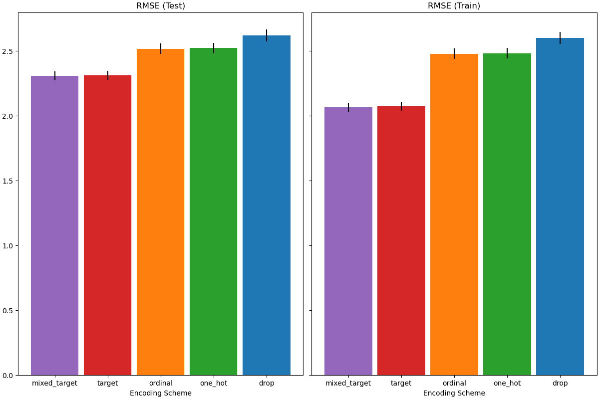
When evaluating the predictive performance on the test set, dropping the categories perform the worst and the target encoders performs the best. This can be explained as follows:
Dropping the categorical features makes the pipeline less expressive and underfitting as a result;
Due to the high cardinality and to reduce the training time, the one-hot encoding scheme uses
max_categories=20which prevents the features from expanding too much, which can result in underfitting.If we had not set
max_categories=20, the one-hot encoding scheme would have likely made the pipeline overfitting as the number of features explodes with rare category occurrences that are correlated with the target by chance (on the training set only);The ordinal encoding imposes an arbitrary order to the features which are then treated as numerical values by the
HistGradientBoostingRegressor. Since this model groups numerical features in 256 bins per feature, many unrelated categories can be grouped together and as a result overall pipeline can underfit;When using the target encoder, the same binning happens, but since the encoded values are statistically ordered by marginal association with the target variable, the binning use by the
HistGradientBoostingRegressormakes sense and leads to good results: the combination of smoothed target encoding and binning works as a good regularizing strategy against overfitting while not limiting the expressiveness of the pipeline too much.
Total running time of the script: (0 minutes 22.439 seconds)
Related examples