Note
Go to the end to download the full example code or to run this example in your browser via JupyterLite or Binder.
Selecting dimensionality reduction with Pipeline and GridSearchCV#
This example constructs a pipeline that does dimensionality
reduction followed by prediction with a support vector
classifier. It demonstrates the use of GridSearchCV and
Pipeline to optimize over different classes of estimators in a
single CV run – unsupervised PCA and NMF dimensionality
reductions are compared to univariate feature selection during
the grid search.
Additionally, Pipeline can be instantiated with the memory
argument to memoize the transformers within the pipeline, avoiding to fit
again the same transformers over and over.
Note that the use of memory to enable caching becomes interesting when the
fitting of a transformer is costly.
# Authors: The scikit-learn developers
# SPDX-License-Identifier: BSD-3-Clause
Illustration of Pipeline and GridSearchCV#
import matplotlib.pyplot as plt
import numpy as np

from sklearn.datasets import load_digits
from sklearn.decomposition import NMF, PCA
from sklearn.feature_selection import SelectKBest, mutual_info_classif
from sklearn.model_selection import GridSearchCV
from sklearn.pipeline import Pipeline
from sklearn.preprocessing import MinMaxScaler
from sklearn.svm import LinearSVC

X, y = load_digits(return_X_y=True)

pipe = Pipeline(
    [
        ("scaling", MinMaxScaler()),
        # the reduce_dim stage is populated by the param_grid
        ("reduce_dim", "passthrough"),
        ("classify", LinearSVC(dual=False, max_iter=10000)),
    ]
)

N_FEATURES_OPTIONS = [2, 4, 8]
C_OPTIONS = [1, 10, 100, 1000]
param_grid = [
    {
        "reduce_dim": [PCA(iterated_power=7), NMF(max_iter=1_000)],
        "reduce_dim__n_components": N_FEATURES_OPTIONS,
        "classify__C": C_OPTIONS,
    },
    {
        "reduce_dim": [SelectKBest(mutual_info_classif)],
        "reduce_dim__k": N_FEATURES_OPTIONS,
        "classify__C": C_OPTIONS,
    },
]
reducer_labels = ["PCA", "NMF", "KBest(mutual_info_classif)"]

grid = GridSearchCV(pipe, n_jobs=1, param_grid=param_grid)
grid.fit(X, y)
GridSearchCV(estimator=Pipeline(steps=[('scaling', MinMaxScaler()),
                                       ('reduce_dim', 'passthrough'),
                                       ('classify',
                                        LinearSVC(dual=False,
                                                  max_iter=10000))]),
             n_jobs=1,
             param_grid=[{'classify__C': [1, 10, 100, 1000],
                          'reduce_dim': [PCA(iterated_power=7),
                                         NMF(max_iter=1000)],
                          'reduce_dim__n_components': [2, 4, 8]},
                         {'classify__C': [1, 10, 100, 1000],
                          'reduce_dim': [SelectKBest(score_func=<function mutual_info_classif at 0x764497121430>)],
                          'reduce_dim__k': [2, 4, 8]}])
In a Jupyter environment, please rerun this cell to show the HTML representation or trust the notebook. On GitHub, the HTML representation is unable to render, please try loading this page with nbviewer.org.
Parameters
Fitted attributes
Parameters
Fitted attributes
64 features
| x0 |
| x1 |
| x2 |
| x3 |
| x4 |
| x5 |
| x6 |
| x7 |
| x8 |
| x9 |
| x10 |
| x11 |
| x12 |
| x13 |
| x14 |
| x15 |
| x16 |
| x17 |
| x18 |
| x19 |
| x20 |
| x21 |
| x22 |
| x23 |
| x24 |
| x25 |
| x26 |
| x27 |
| x28 |
| x29 |
| x30 |
| x31 |
| x32 |
| x33 |
| x34 |
| x35 |
| x36 |
| x37 |
| x38 |
| x39 |
| x40 |
| x41 |
| x42 |
| x43 |
| x44 |
| x45 |
| x46 |
| x47 |
| x48 |
| x49 |
| x50 |
| x51 |
| x52 |
| x53 |
| x54 |
| x55 |
| x56 |
| x57 |
| x58 |
| x59 |
| x60 |
| x61 |
| x62 |
| x63 |
Parameters
Fitted attributes
8 features
| pca0 |
| pca1 |
| pca2 |
| pca3 |
| pca4 |
| pca5 |
| pca6 |
| pca7 |
Parameters
Fitted attributes
import pandas as pd
mean_scores = np.array(grid.cv_results_["mean_test_score"])
# scores are in the order of param_grid iteration, which is alphabetical
mean_scores = mean_scores.reshape(len(C_OPTIONS), -1, len(N_FEATURES_OPTIONS))
# select score for best C
mean_scores = mean_scores.max(axis=0)
# create a dataframe to ease plotting
mean_scores = pd.DataFrame(
mean_scores.T, index=N_FEATURES_OPTIONS, columns=reducer_labels
)
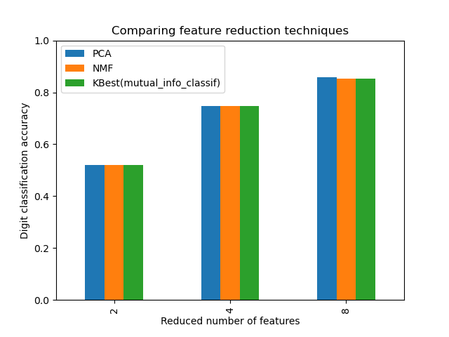
ax = mean_scores.plot.bar()
ax.set_title("Comparing feature reduction techniques")
ax.set_xlabel("Reduced number of features")
ax.set_ylabel("Digit classification accuracy")
ax.set_ylim((0, 1))
ax.legend(loc="upper left")
plt.show()
Caching transformers within a Pipeline#
It is sometimes worthwhile storing the state of a specific transformer
since it could be used again. Using a pipeline in GridSearchCV triggers
such situations. Therefore, we use the argument memory to enable caching.
Warning
Note that this example is, however, only an illustration since for this
specific case fitting PCA is not necessarily slower than loading the
cache. Hence, use the memory constructor parameter when the fitting
of a transformer is costly.
from shutil import rmtree

from joblib import Memory

# Create a temporary folder to store the transformers of the pipeline
location = "cachedir"
memory = Memory(location=location, verbose=10)
cached_pipe = Pipeline(
    [("reduce_dim", PCA()), ("classify", LinearSVC(dual=False, max_iter=10000))],
    memory=memory,
)

# This time, a cached pipeline will be used within the grid search


# Delete the temporary cache before exiting
memory.clear(warn=False)
rmtree(location)
The PCA fitting is only computed at the evaluation of the first
configuration of the C parameter of the LinearSVC classifier. The
other configurations of C will trigger the loading of the cached PCA
estimator data, leading to save processing time. Therefore, the use of
caching the pipeline using memory is highly beneficial when fitting
a transformer is costly.
Total running time of the script: (0 minutes 56.026 seconds)
Related examples