Note
Go to the end to download the full example code or to run this example in your browser via JupyterLite or Binder.
Demo of HDBSCAN clustering algorithm#
In this demo we will take a look at cluster.HDBSCAN from the
perspective of generalizing the cluster.DBSCAN algorithm.
We’ll compare both algorithms on specific datasets. Finally we’ll evaluate
HDBSCAN’s sensitivity to certain hyperparameters.
We first define a couple utility functions for convenience.
# Authors: The scikit-learn developers
# SPDX-License-Identifier: BSD-3-Clause
import matplotlib.pyplot as plt
import numpy as np

from sklearn.cluster import DBSCAN, HDBSCAN
from sklearn.datasets import make_blobs


def plot(X, labels, probabilities=None, parameters=None, ground_truth=False, ax=None):
    if ax is None:
        _, ax = plt.subplots(figsize=(10, 4))
    labels = labels if labels is not None else np.ones(X.shape[0])
    probabilities = probabilities if probabilities is not None else np.ones(X.shape[0])
    # Black removed and is used for noise instead.
    unique_labels = set(labels)
    colors = [plt.cm.Spectral(each) for each in np.linspace(0, 1, len(unique_labels))]
    # The probability of a point belonging to its labeled cluster determines
    # the size of its marker
    proba_map = {idx: probabilities[idx] for idx in range(len(labels))}
    for k, col in zip(unique_labels, colors):
        if k == -1:
            # Black used for noise.
            col = [0, 0, 0, 1]

        class_index = (labels == k).nonzero()[0]
        for ci in class_index:
            ax.plot(
                X[ci, 0],
                X[ci, 1],
                "x" if k == -1 else "o",
                markerfacecolor=tuple(col),
                markeredgecolor="k",
                markersize=4 if k == -1 else 1 + 5 * proba_map[ci],
            )
    n_clusters_ = len(set(labels)) - (1 if -1 in labels else 0)
    preamble = "True" if ground_truth else "Estimated"
    title = f"{preamble} number of clusters: {n_clusters_}"
    if parameters is not None:
        parameters_str = ", ".join(f"{k}={v}" for k, v in parameters.items())
        title += f" | {parameters_str}"
    ax.set_title(title)
    plt.tight_layout()
Generate sample data#
One of the greatest advantages of HDBSCAN over DBSCAN is its out-of-the-box
robustness. It’s especially remarkable on heterogeneous mixtures of data.
Like DBSCAN, it can model arbitrary shapes and distributions, however unlike
DBSCAN it does not require specification of an arbitrary and sensitive
eps hyperparameter.
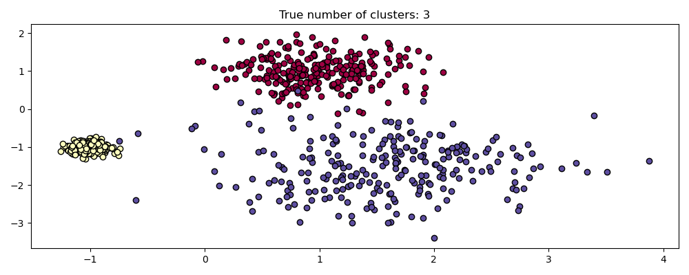
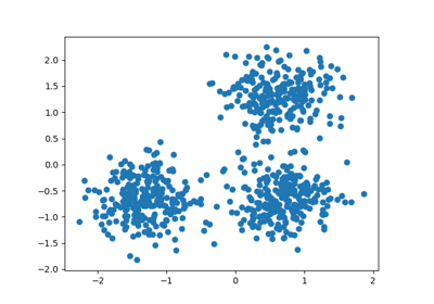
For example, below we generate a dataset from a mixture of three bi-dimensional and isotropic Gaussian distributions.
centers = [[1, 1], [-1, -1], [1.5, -1.5]]
X, labels_true = make_blobs(
    n_samples=750, centers=centers, cluster_std=[0.4, 0.1, 0.75], random_state=0
)
plot(X, labels=labels_true, ground_truth=True)
Scale Invariance#
It’s worth remembering that, while DBSCAN provides a default value for eps
parameter, it hardly has a proper default value and must be tuned for the
specific dataset at use.
As a simple demonstration, consider the clustering for a eps value tuned
for one dataset, and clustering obtained with the same value but applied to
rescaled versions of the dataset.
fig, axes = plt.subplots(3, 1, figsize=(10, 12))
dbs = DBSCAN(eps=0.3)
for idx, scale in enumerate([1, 0.5, 3]):
    dbs.fit(X * scale)
    plot(X * scale, dbs.labels_, parameters={"scale": scale, "eps": 0.3}, ax=axes[idx])
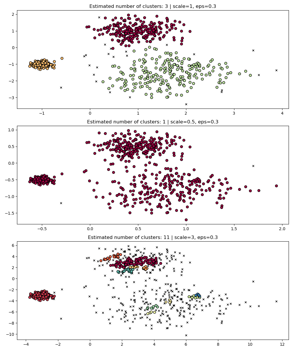
Indeed, in order to maintain the same results we would have to scale eps by
the same factor.
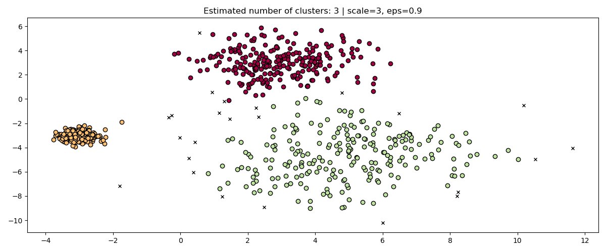
fig, axis = plt.subplots(1, 1, figsize=(12, 5))
dbs = DBSCAN(eps=0.9).fit(3 * X)
plot(3 * X, dbs.labels_, parameters={"scale": 3, "eps": 0.9}, ax=axis)
While standardizing data (e.g. using
sklearn.preprocessing.StandardScaler) helps mitigate this problem,
great care must be taken to select the appropriate value for eps.
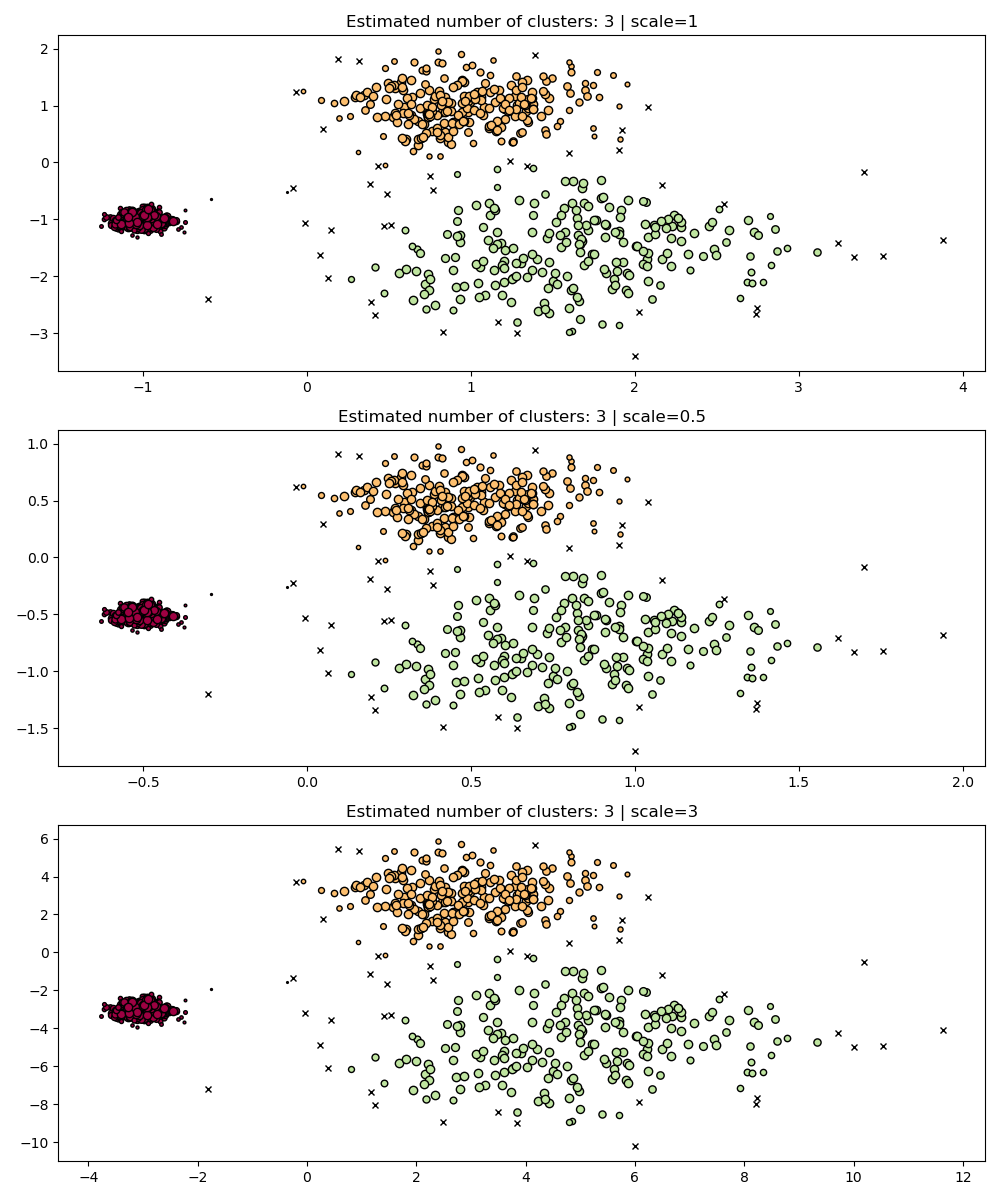
HDBSCAN is much more robust in this sense: HDBSCAN can be seen as
clustering over all possible values of eps and extracting the best
clusters from all possible clusters (see User Guide).
One immediate advantage is that HDBSCAN is scale-invariant.
fig, axes = plt.subplots(3, 1, figsize=(10, 12))
hdb = HDBSCAN(copy=True)
for idx, scale in enumerate([1, 0.5, 3]):
    hdb.fit(X * scale)
    plot(
        X * scale,
        hdb.labels_,
        hdb.probabilities_,
        ax=axes[idx],
        parameters={"scale": scale},
    )
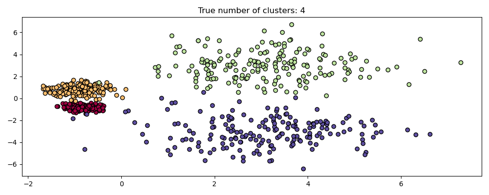
Multi-Scale Clustering#
HDBSCAN is much more than scale invariant though – it is capable of multi-scale clustering, which accounts for clusters with varying density. Traditional DBSCAN assumes that any potential clusters are homogeneous in density. HDBSCAN is free from such constraints. To demonstrate this we consider the following dataset
centers = [[-0.85, -0.85], [-0.85, 0.85], [3, 3], [3, -3]]
X, labels_true = make_blobs(
    n_samples=750, centers=centers, cluster_std=[0.2, 0.35, 1.35, 1.35], random_state=0
)
plot(X, labels=labels_true, ground_truth=True)
This dataset is more difficult for DBSCAN due to the varying densities and spatial separation:
If
epsis too large then we risk falsely clustering the two dense clusters as one since their mutual reachability will extend clusters.If
epsis too small, then we risk fragmenting the sparser clusters into many false clusters.
Not to mention this requires manually tuning choices of eps until we
find a tradeoff that we are comfortable with.
fig, axes = plt.subplots(2, 1, figsize=(10, 8))
params = {"eps": 0.7}
dbs = DBSCAN(**params).fit(X)
plot(X, dbs.labels_, parameters=params, ax=axes[0])
params = {"eps": 0.3}
dbs = DBSCAN(**params).fit(X)
plot(X, dbs.labels_, parameters=params, ax=axes[1])
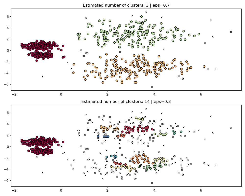
To properly cluster the two dense clusters, we would need a smaller value of
epsilon, however at eps=0.3 we are already fragmenting the sparse clusters,
which would only become more severe as we decrease epsilon. Indeed it seems
that DBSCAN is incapable of simultaneously separating the two dense clusters
while preventing the sparse clusters from fragmenting. Let’s compare with
HDBSCAN.
hdb = HDBSCAN(copy=True).fit(X)
plot(X, hdb.labels_, hdb.probabilities_)
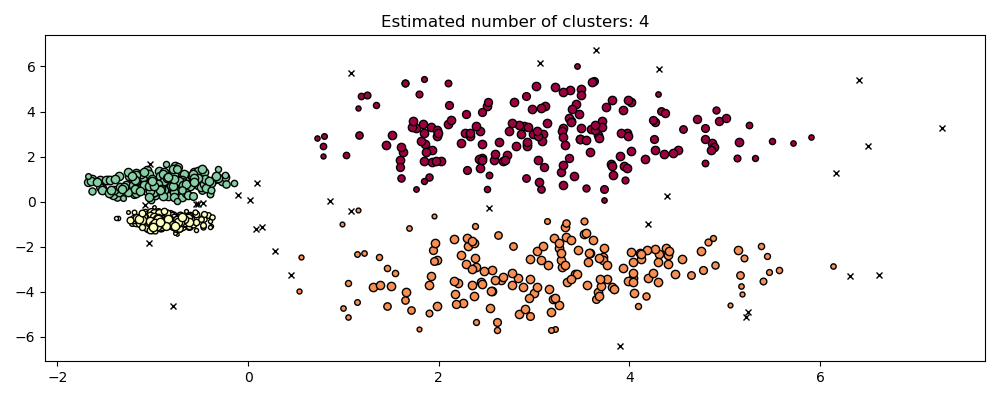
HDBSCAN is able to adapt to the multi-scale structure of the dataset without requiring parameter tuning. While any sufficiently interesting dataset will require tuning, this case demonstrates that HDBSCAN can yield qualitatively better classes of clusterings without users’ intervention which are inaccessible via DBSCAN.
Hyperparameter Robustness#
Ultimately tuning will be an important step in any real world application, so
let’s take a look at some of the most important hyperparameters for HDBSCAN.
While HDBSCAN is free from the eps parameter of DBSCAN, it does still have
some hyperparameters like min_cluster_size and min_samples which tune its
results regarding density. We will however see that HDBSCAN is relatively robust
to various real world examples thanks to those parameters whose clear meaning
helps tuning them.
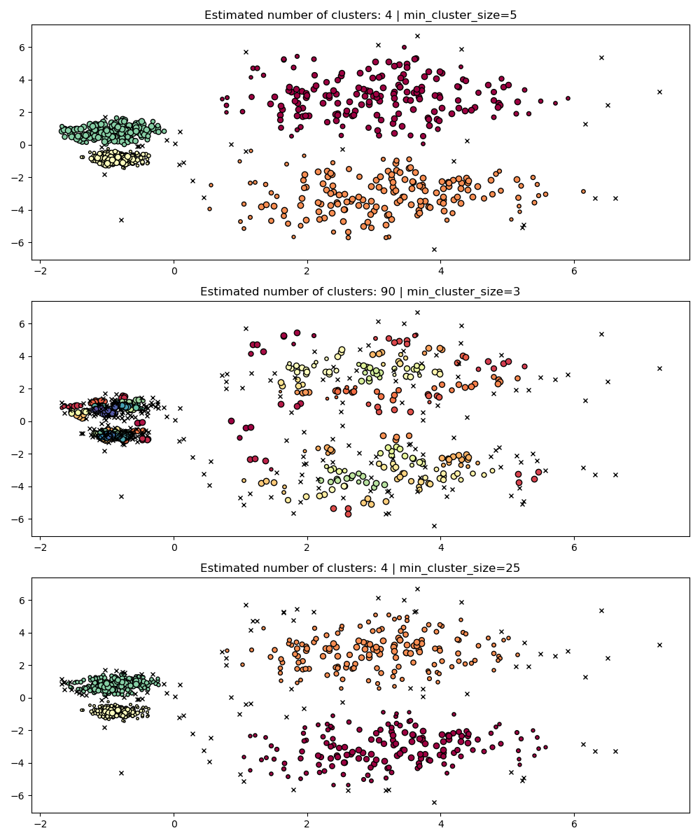
min_cluster_size#
min_cluster_size is the minimum number of samples in a group for that
group to be considered a cluster.
Clusters smaller than the ones of this size will be left as noise. The default value is 5. This parameter is generally tuned to larger values as needed. Smaller values will likely to lead to results with fewer points labeled as noise. However values which too small will lead to false sub-clusters being picked up and preferred. Larger values tend to be more robust with respect to noisy datasets, e.g. high-variance clusters with significant overlap.
PARAM = ({"min_cluster_size": 5}, {"min_cluster_size": 3}, {"min_cluster_size": 25})
fig, axes = plt.subplots(3, 1, figsize=(10, 12))
for i, param in enumerate(PARAM):
    hdb = HDBSCAN(copy=True, **param).fit(X)
    labels = hdb.labels_

    plot(X, labels, hdb.probabilities_, param, ax=axes[i])
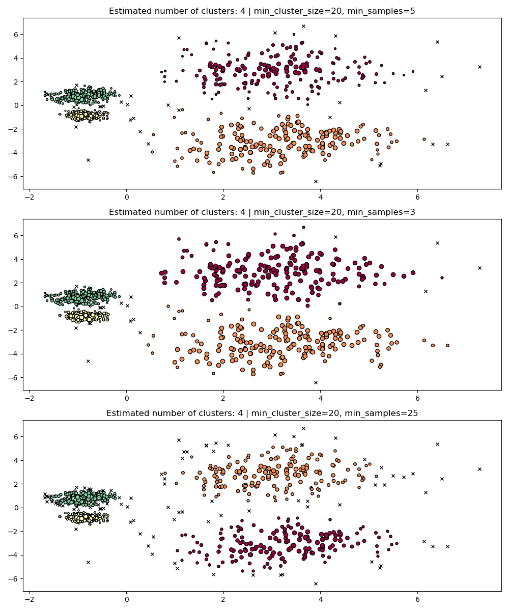
min_samples#
min_samples is the number of samples in a neighborhood for a point to
be considered as a core point, including the point itself.
min_samples defaults to min_cluster_size.
Similarly to min_cluster_size, larger values for min_samples increase
the model’s robustness to noise, but risks ignoring or discarding
potentially valid but small clusters.
min_samples better be tuned after finding a good value for min_cluster_size.
PARAM = (
    {"min_cluster_size": 20, "min_samples": 5},
    {"min_cluster_size": 20, "min_samples": 3},
    {"min_cluster_size": 20, "min_samples": 25},
)
fig, axes = plt.subplots(3, 1, figsize=(10, 12))
for i, param in enumerate(PARAM):
    hdb = HDBSCAN(copy=True, **param).fit(X)
    labels = hdb.labels_

    plot(X, labels, hdb.probabilities_, param, ax=axes[i])
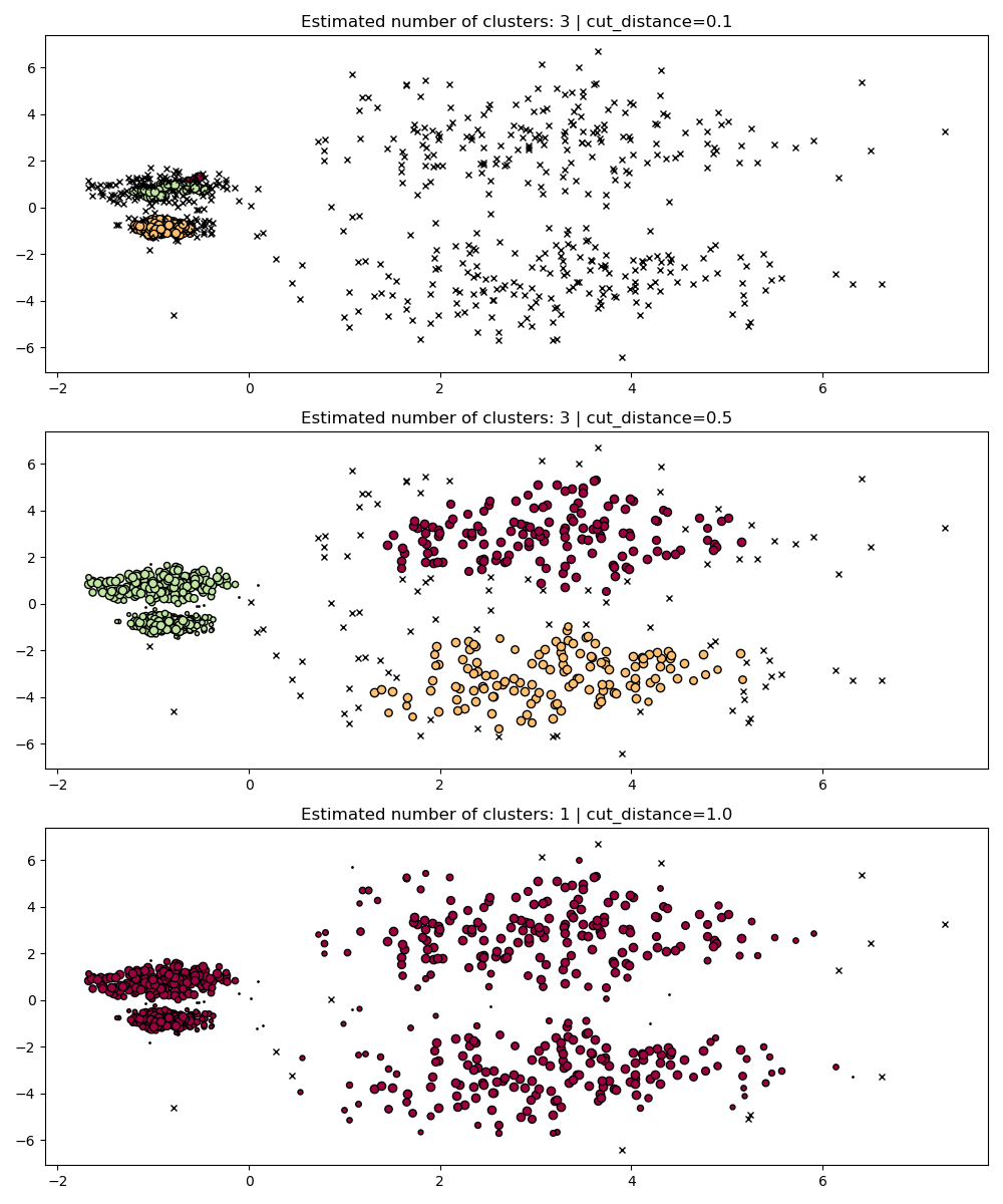
dbscan_clustering#
During fit, HDBSCAN builds a single-linkage tree which encodes the
clustering of all points across all values of DBSCAN’s
eps parameter.
We can thus plot and evaluate these clusterings efficiently without fully
recomputing intermediate values such as core-distances, mutual-reachability,
and the minimum spanning tree. All we need to do is specify the cut_distance
(equivalent to eps) we want to cluster with.
PARAM = (
    {"cut_distance": 0.1},
    {"cut_distance": 0.5},
    {"cut_distance": 1.0},
)
hdb = HDBSCAN(copy=True)
hdb.fit(X)
fig, axes = plt.subplots(len(PARAM), 1, figsize=(10, 12))
for i, param in enumerate(PARAM):
    labels = hdb.dbscan_clustering(**param)

    plot(X, labels, hdb.probabilities_, param, ax=axes[i])
Total running time of the script: (0 minutes 16.338 seconds)
Related examples
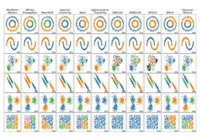
Comparing different clustering algorithms on toy datasets
The Johnson-Lindenstrauss bound for embedding with random projections
