L1-based models for Sparse Signals

The present example compares three l1-based regression models on a synthetic signal obtained from sparse and correlated features that are further corrupted with additive gaussian noise:

• a Lasso;

• an Automatic Relevance Determination - ARD;

• an Elastic-Net.

It is known that the Lasso estimates turn to be close to the model selection estimates when the data dimensions grow, given that the irrelevant variables are not too correlated with the relevant ones. In the presence of correlated features, Lasso itself cannot select the correct sparsity pattern [1].

Here we compare the performance of the three models in terms of the \(R^2\) score, the fitting time and the sparsity of the estimated coefficients when compared with the ground-truth.

# Author: Arturo Amor <david-arturo.amor-quiroz@inria.fr>

Generate synthetic dataset

We generate a dataset where the number of samples is lower than the total number of features. This leads to an underdetermined system, i.e. the solution is not unique, and thus we cannot apply an Ordinary Least Squares by itself. Regularization introduces a penalty term to the objective function, which modifies the optimization problem and can help alleviate the underdetermined nature of the system.

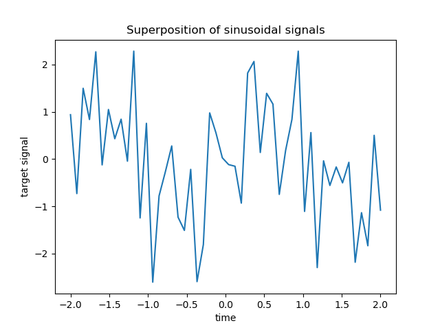
The target y is a linear combination with alternating signs of sinusoidal signals. Only the 10 lowest out of the 100 frequencies in X are used to generate y, while the rest of the features are not informative. This results in a high dimensional sparse feature space, where some degree of l1-penalization is necessary.

import numpy as np

rng = np.random.RandomState(0)
n_samples, n_features, n_informative = 50, 100, 10
time_step = np.linspace(-2, 2, n_samples)
freqs = 2 * np.pi * np.sort(rng.rand(n_features)) / 0.01
X = np.zeros((n_samples, n_features))

for i in range(n_features):
    X[:, i] = np.sin(freqs[i] * time_step)

idx = np.arange(n_features)
true_coef = (-1) ** idx * np.exp(-idx / 10)
true_coef[n_informative:] = 0  # sparsify coef
y = np.dot(X, true_coef)

Some of the informative features have close frequencies to induce (anti-)correlations.

freqs[:n_informative]

array([ 2.9502547 , 11.8059798 , 12.63394388, 12.70359377, 24.62241605,
       37.84077985, 40.30506066, 44.63327171, 54.74495357, 59.02456369])

A random phase is introduced using numpy.random.random_sample and some gaussian noise (implemented by numpy.random.normal) is added to both the features and the target.

for i in range(n_features):
    X[:, i] = np.sin(freqs[i] * time_step + 2 * (rng.random_sample() - 0.5))
    X[:, i] += 0.2 * rng.normal(0, 1, n_samples)

y += 0.2 * rng.normal(0, 1, n_samples)

Such sparse, noisy and correlated features can be obtained, for instance, from sensor nodes monitoring some environmental variables, as they typically register similar values depending on their positions (spatial correlations). We can visualize the target.

import matplotlib.pyplot as plt

plt.plot(time_step, y)
plt.ylabel("target signal")
plt.xlabel("time")
_ = plt.title("Superposition of sinusoidal signals")

We split the data into train and test sets for simplicity. In practice one should use a TimeSeriesSplit cross-validation to estimate the variance of the test score. Here we set shuffle="False" as we must not use training data that succeed the testing data when dealing with data that have a temporal relationship.

from sklearn.model_selection import train_test_split

X_train, X_test, y_train, y_test = train_test_split(X, y, test_size=0.5, shuffle=False)

In the following, we compute the performance of three l1-based models in terms of the goodness of fit \(R^2\) score and the fitting time. Then we make a plot to compare the sparsity of the estimated coefficients with respect to the ground-truth coefficients and finally we analyze the previous results.

Lasso

In this example, we demo a Lasso with a fixed value of the regularization parameter alpha. In practice, the optimal parameter alpha should be selected by passing a TimeSeriesSplit cross-validation strategy to a LassoCV. To keep the example simple and fast to execute, we directly set the optimal value for alpha here.

from time import time

from sklearn.linear_model import Lasso
from sklearn.metrics import r2_score

t0 = time()
lasso = Lasso(alpha=0.14).fit(X_train, y_train)
print(f"Lasso fit done in {(time() - t0):.3f}s")

y_pred_lasso = lasso.predict(X_test)
r2_score_lasso = r2_score(y_test, y_pred_lasso)
print(f"Lasso r^2 on test data : {r2_score_lasso:.3f}")

Lasso fit done in 0.001s
Lasso r^2 on test data : 0.480

Automatic Relevance Determination (ARD)

An ARD regression is the bayesian version of the Lasso. It can produce interval estimates for all of the parameters, including the error variance, if required. It is a suitable option when the signals have gaussian noise. See the example Comparing Linear Bayesian Regressors for a comparison of ARDRegression and BayesianRidge regressors.

from sklearn.linear_model import ARDRegression

t0 = time()
ard = ARDRegression().fit(X_train, y_train)
print(f"ARD fit done in {(time() - t0):.3f}s")

y_pred_ard = ard.predict(X_test)
r2_score_ard = r2_score(y_test, y_pred_ard)
print(f"ARD r^2 on test data : {r2_score_ard:.3f}")

ARD fit done in 0.012s
ARD r^2 on test data : 0.543

ElasticNet

ElasticNet is a middle ground between Lasso and Ridge, as it combines a L1 and a L2-penalty. The amount of regularization is controlled by the two hyperparameters l1_ratio and alpha. For l1_ratio = 0 the penalty is pure L2 and the model is equivalent to a Ridge. Similarly, l1_ratio = 1 is a pure L1 penalty and the model is equivalent to a Lasso. For 0 < l1_ratio < 1, the penalty is a combination of L1 and L2.

As done before, we train the model with fix values for alpha and l1_ratio. To select their optimal value we used an ElasticNetCV, not shown here to keep the example simple.

from sklearn.linear_model import ElasticNet

t0 = time()
enet = ElasticNet(alpha=0.08, l1_ratio=0.5).fit(X_train, y_train)
print(f"ElasticNet fit done in {(time() - t0):.3f}s")

y_pred_enet = enet.predict(X_test)
r2_score_enet = r2_score(y_test, y_pred_enet)
print(f"ElasticNet r^2 on test data : {r2_score_enet:.3f}")

ElasticNet fit done in 0.001s
ElasticNet r^2 on test data : 0.636

Plot and analysis of the results

In this section, we use a heatmap to visualize the sparsity of the true and estimated coefficients of the respective linear models.

import matplotlib.pyplot as plt
import pandas as pd
import seaborn as sns
from matplotlib.colors import SymLogNorm

df = pd.DataFrame(
    {
        "True coefficients": true_coef,
        "Lasso": lasso.coef_,
        "ARDRegression": ard.coef_,
        "ElasticNet": enet.coef_,
    }
)

plt.figure(figsize=(10, 6))
ax = sns.heatmap(
    df.T,
    norm=SymLogNorm(linthresh=10e-4, vmin=-1, vmax=1),
    cbar_kws={"label": "coefficients' values"},
    cmap="seismic_r",
)
plt.ylabel("linear model")
plt.xlabel("coefficients")
plt.title(
    f"Models' coefficients\nLasso $R^2$: {r2_score_lasso:.3f}, "
    f"ARD $R^2$: {r2_score_ard:.3f}, "
    f"ElasticNet $R^2$: {r2_score_enet:.3f}"
)
plt.tight_layout()

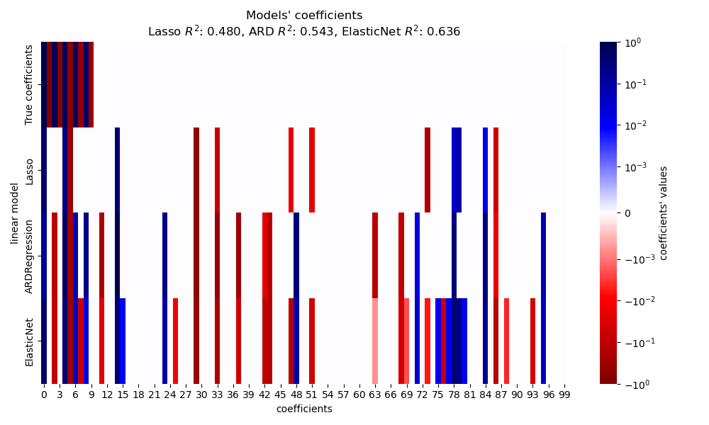
In the present example ElasticNet yields the best score and captures the most of the predictive features, yet still fails at finding all the true components. Notice that both ElasticNet and ARDRegression result in a less sparse model than a Lasso.

Conclusions

Lasso is known to recover sparse data effectively but does not perform well with highly correlated features. Indeed, if several correlated features contribute to the target, Lasso would end up selecting a single one of them. In the case of sparse yet non-correlated features, a Lasso model would be more suitable.

ElasticNet introduces some sparsity on the coefficients and shrinks their values to zero. Thus, in the presence of correlated features that contribute to the target, the model is still able to reduce their weights without setting them exactly to zero. This results in a less sparse model than a pure Lasso and may capture non-predictive features as well.

ARDRegression is better when handling gaussian noise, but is still unable to handle correlated features and requires a larger amount of time due to fitting a prior.

References

[1]

“Lasso-type recovery of sparse representations for high-dimensional data” N. Meinshausen, B. Yu - The Annals of Statistics 2009, Vol. 37, No. 1, 246-270

Related examples

Lasso on dense and sparse data

Lasso on dense and sparse data

Joint feature selection with multi-task Lasso

Joint feature selection with multi-task Lasso

Lasso model selection: AIC-BIC / cross-validation

Lasso model selection: AIC-BIC / cross-validation

Lasso and Elastic Net

Lasso and Elastic Net

Comparing Linear Bayesian Regressors

Comparing Linear Bayesian Regressors