Note
Go to the end to download the full example code or to run this example in your browser via JupyterLite or Binder.
Gradient Boosting regularization#
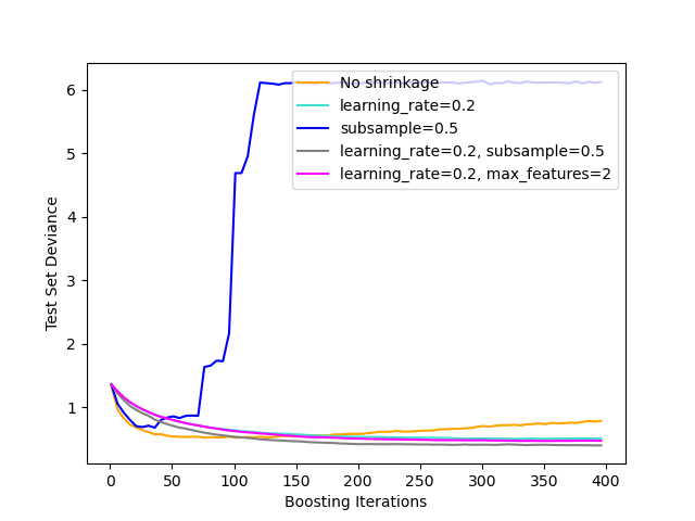
Illustration of the effect of different regularization strategies for Gradient Boosting. The example is taken from Hastie et al 2009 [1].
The loss function used is binomial deviance. Regularization via
shrinkage (learning_rate < 1.0) improves performance considerably.
In combination with shrinkage, stochastic gradient boosting
(subsample < 1.0) can produce more accurate models by reducing the
variance via bagging.
Subsampling without shrinkage usually does poorly.
Another strategy to reduce the variance is by subsampling the features
analogous to the random splits in Random Forests
(via the max_features parameter).
# Authors: The scikit-learn developers
# SPDX-License-Identifier: BSD-3-Clause

import matplotlib.pyplot as plt
import numpy as np

from sklearn import datasets, ensemble
from sklearn.metrics import log_loss
from sklearn.model_selection import train_test_split

X, y = datasets.make_hastie_10_2(n_samples=4000, random_state=1)

# map labels from {-1, 1} to {0, 1}
labels, y = np.unique(y, return_inverse=True)

X_train, X_test, y_train, y_test = train_test_split(X, y, test_size=0.8, random_state=0)

original_params = {
    "n_estimators": 400,
    "max_leaf_nodes": 4,
    "max_depth": None,
    "random_state": 2,
    "min_samples_split": 5,
}

plt.figure()

for label, color, setting in [
    ("No shrinkage", "orange", {"learning_rate": 1.0, "subsample": 1.0}),
    ("learning_rate=0.2", "turquoise", {"learning_rate": 0.2, "subsample": 1.0}),
    ("subsample=0.5", "blue", {"learning_rate": 1.0, "subsample": 0.5}),
    (
        "learning_rate=0.2, subsample=0.5",
        "gray",
        {"learning_rate": 0.2, "subsample": 0.5},
    ),
    (
        "learning_rate=0.2, max_features=2",
        "magenta",
        {"learning_rate": 0.2, "max_features": 2},
    ),
]:
    params = dict(original_params)
    params.update(setting)

    clf = ensemble.GradientBoostingClassifier(**params)
    clf.fit(X_train, y_train)

    # compute test set deviance
    test_deviance = np.zeros((params["n_estimators"],), dtype=np.float64)

    for i, y_proba in enumerate(clf.staged_predict_proba(X_test)):
        test_deviance[i] = 2 * log_loss(y_test, y_proba[:, 1])

    plt.plot(
        (np.arange(test_deviance.shape[0]) + 1)[::5],
        test_deviance[::5],
        "-",
        color=color,
        label=label,
    )

plt.legend(loc="upper right")
plt.xlabel("Boosting Iterations")
plt.ylabel("Test Set Deviance")

plt.show()
Total running time of the script: (0 minutes 7.203 seconds)
Related examples
Compare Stochastic learning strategies for MLPClassifier
Shrinkage covariance estimation: LedoitWolf vs OAS and max-likelihood
