Note

Go to the end to download the full example code. or to run this example in your browser via JupyterLite or Binder

t-SNE: The effect of various perplexity values on the shape#

An illustration of t-SNE on the two concentric circles and the S-curve datasets for different perplexity values.

We observe a tendency towards clearer shapes as the perplexity value increases.

The size, the distance and the shape of clusters may vary upon initialization, perplexity values and does not always convey a meaning.

As shown below, t-SNE for higher perplexities finds meaningful topology of two concentric circles, however the size and the distance of the circles varies slightly from the original. Contrary to the two circles dataset, the shapes visually diverge from S-curve topology on the S-curve dataset even for larger perplexity values.

For further details, “How to Use t-SNE Effectively” https://distill.pub/2016/misread-tsne/ provides a good discussion of the effects of various parameters, as well as interactive plots to explore those effects.

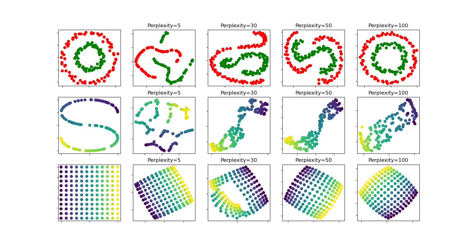
Perplexity=5, Perplexity=30, Perplexity=50, Perplexity=100, Perplexity=5, Perplexity=30, Perplexity=50, Perplexity=100, Perplexity=5, Perplexity=30, Perplexity=50, Perplexity=100

circles, perplexity=5 in 0.13 sec
circles, perplexity=30 in 0.21 sec
circles, perplexity=50 in 0.23 sec
circles, perplexity=100 in 0.23 sec
S-curve, perplexity=5 in 0.13 sec
S-curve, perplexity=30 in 0.19 sec
S-curve, perplexity=50 in 0.23 sec
S-curve, perplexity=100 in 0.23 sec
uniform grid, perplexity=5 in 0.16 sec
uniform grid, perplexity=30 in 0.23 sec
uniform grid, perplexity=50 in 0.26 sec
uniform grid, perplexity=100 in 0.27 sec

# Authors: The scikit-learn developers
# SPDX-License-Identifier: BSD-3-Clause

from time import time

import matplotlib.pyplot as plt
import numpy as np
from matplotlib.ticker import NullFormatter

from sklearn import datasets, manifold

n_samples = 150
n_components = 2
(fig, subplots) = plt.subplots(3, 5, figsize=(15, 8))
perplexities = [5, 30, 50, 100]

X, y = datasets.make_circles(
    n_samples=n_samples, factor=0.5, noise=0.05, random_state=0
)

red = y == 0
green = y == 1

ax = subplots[0][0]
ax.scatter(X[red, 0], X[red, 1], c="r")
ax.scatter(X[green, 0], X[green, 1], c="g")
ax.xaxis.set_major_formatter(NullFormatter())
ax.yaxis.set_major_formatter(NullFormatter())
plt.axis("tight")

for i, perplexity in enumerate(perplexities):
    ax = subplots[0][i + 1]

    t0 = time()
    tsne = manifold.TSNE(
        n_components=n_components,
        init="random",
        random_state=0,
        perplexity=perplexity,
        max_iter=300,
    )
    Y = tsne.fit_transform(X)
    t1 = time()
    print("circles, perplexity=%d in %.2g sec" % (perplexity, t1 - t0))
    ax.set_title("Perplexity=%d" % perplexity)
    ax.scatter(Y[red, 0], Y[red, 1], c="r")
    ax.scatter(Y[green, 0], Y[green, 1], c="g")
    ax.xaxis.set_major_formatter(NullFormatter())
    ax.yaxis.set_major_formatter(NullFormatter())
    ax.axis("tight")

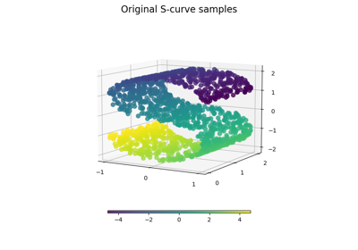
# Another example using s-curve
X, color = datasets.make_s_curve(n_samples, random_state=0)

ax = subplots[1][0]
ax.scatter(X[:, 0], X[:, 2], c=color)
ax.xaxis.set_major_formatter(NullFormatter())
ax.yaxis.set_major_formatter(NullFormatter())

for i, perplexity in enumerate(perplexities):
    ax = subplots[1][i + 1]

    t0 = time()
    tsne = manifold.TSNE(
        n_components=n_components,
        init="random",
        random_state=0,
        perplexity=perplexity,
        learning_rate="auto",
        max_iter=300,
    )
    Y = tsne.fit_transform(X)
    t1 = time()
    print("S-curve, perplexity=%d in %.2g sec" % (perplexity, t1 - t0))

    ax.set_title("Perplexity=%d" % perplexity)
    ax.scatter(Y[:, 0], Y[:, 1], c=color)
    ax.xaxis.set_major_formatter(NullFormatter())
    ax.yaxis.set_major_formatter(NullFormatter())
    ax.axis("tight")


# Another example using a 2D uniform grid
x = np.linspace(0, 1, int(np.sqrt(n_samples)))
xx, yy = np.meshgrid(x, x)
X = np.hstack(
    [
        xx.ravel().reshape(-1, 1),
        yy.ravel().reshape(-1, 1),
    ]
)
color = xx.ravel()
ax = subplots[2][0]
ax.scatter(X[:, 0], X[:, 1], c=color)
ax.xaxis.set_major_formatter(NullFormatter())
ax.yaxis.set_major_formatter(NullFormatter())

for i, perplexity in enumerate(perplexities):
    ax = subplots[2][i + 1]

    t0 = time()
    tsne = manifold.TSNE(
        n_components=n_components,
        init="random",
        random_state=0,
        perplexity=perplexity,
        max_iter=400,
    )
    Y = tsne.fit_transform(X)
    t1 = time()
    print("uniform grid, perplexity=%d in %.2g sec" % (perplexity, t1 - t0))

    ax.set_title("Perplexity=%d" % perplexity)
    ax.scatter(Y[:, 0], Y[:, 1], c=color)
    ax.xaxis.set_major_formatter(NullFormatter())
    ax.yaxis.set_major_formatter(NullFormatter())
    ax.axis("tight")


plt.show()