Note
Go to the end to download the full example code or to run this example in your browser via JupyterLite or Binder.
Using KBinsDiscretizer to discretize continuous features#
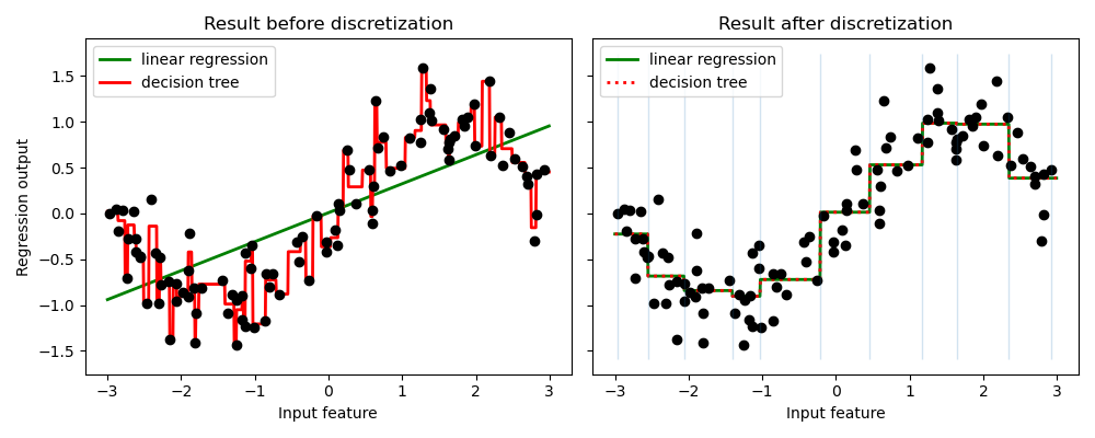
The example compares prediction result of linear regression (linear model) and decision tree (tree based model) with and without discretization of real-valued features.
As is shown in the result before discretization, linear model is fast to build and relatively straightforward to interpret, but can only model linear relationships, while decision tree can build a much more complex model of the data. One way to make linear model more powerful on continuous data is to use discretization (also known as binning). In the example, we discretize the feature and one-hot encode the transformed data. Note that if the bins are not reasonably wide, there would appear to be a substantially increased risk of overfitting, so the discretizer parameters should usually be tuned under cross validation.
After discretization, linear regression and decision tree make exactly the same prediction. As features are constant within each bin, any model must predict the same value for all points within a bin. Compared with the result before discretization, linear model become much more flexible while decision tree gets much less flexible. Note that binning features generally has no beneficial effect for tree-based models, as these models can learn to split up the data anywhere.
# Authors: The scikit-learn developers
# SPDX-License-Identifier: BSD-3-Clause

import matplotlib.pyplot as plt
import numpy as np

from sklearn.linear_model import LinearRegression
from sklearn.preprocessing import KBinsDiscretizer
from sklearn.tree import DecisionTreeRegressor

# construct the dataset
rnd = np.random.RandomState(42)
X = rnd.uniform(-3, 3, size=100)
y = np.sin(X) + rnd.normal(size=len(X)) / 3
X = X.reshape(-1, 1)

# transform the dataset with KBinsDiscretizer
enc = KBinsDiscretizer(
    n_bins=10, encode="onehot", quantile_method="averaged_inverted_cdf"
)
X_binned = enc.fit_transform(X)

# predict with original dataset
fig, (ax1, ax2) = plt.subplots(ncols=2, sharey=True, figsize=(10, 4))
line = np.linspace(-3, 3, 1000, endpoint=False).reshape(-1, 1)
reg = LinearRegression().fit(X, y)
ax1.plot(line, reg.predict(line), linewidth=2, color="green", label="linear regression")
reg = DecisionTreeRegressor(min_samples_split=3, random_state=0).fit(X, y)
ax1.plot(line, reg.predict(line), linewidth=2, color="red", label="decision tree")
ax1.plot(X[:, 0], y, "o", c="k")
ax1.legend(loc="best")
ax1.set_ylabel("Regression output")
ax1.set_xlabel("Input feature")
ax1.set_title("Result before discretization")

# predict with transformed dataset
line_binned = enc.transform(line)
reg = LinearRegression().fit(X_binned, y)
ax2.plot(
    line,
    reg.predict(line_binned),
    linewidth=2,
    color="green",
    linestyle="-",
    label="linear regression",
)
reg = DecisionTreeRegressor(min_samples_split=3, random_state=0).fit(X_binned, y)
ax2.plot(
    line,
    reg.predict(line_binned),
    linewidth=2,
    color="red",
    linestyle=":",
    label="decision tree",
)
ax2.plot(X[:, 0], y, "o", c="k")
ax2.vlines(enc.bin_edges_[0], *plt.gca().get_ylim(), linewidth=1, alpha=0.2)
ax2.legend(loc="best")
ax2.set_xlabel("Input feature")
ax2.set_title("Result after discretization")

plt.tight_layout()
plt.show()
Total running time of the script: (0 minutes 0.218 seconds)
Related examples
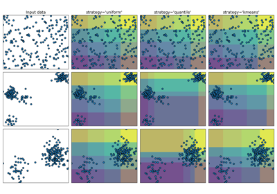
Demonstrating the different strategies of KBinsDiscretizer