Note
Go to the end to download the full example code or to run this example in your browser via JupyterLite or Binder.
Prediction Intervals for Gradient Boosting Regression#
This example shows how quantile regression can be used to create prediction
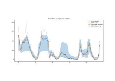
intervals. See Features in Histogram Gradient Boosting Trees
for an example showcasing some other features of
HistGradientBoostingRegressor.
# Authors: The scikit-learn developers
# SPDX-License-Identifier: BSD-3-Clause
Generate some data for a synthetic regression problem by applying the function f to uniformly sampled random inputs.
import numpy as np

from sklearn.model_selection import train_test_split


def f(x):
    """The function to predict."""
    return x * np.sin(x)


rng = np.random.RandomState(42)
X = np.atleast_2d(rng.uniform(0, 10.0, size=1000)).T
expected_y = f(X).ravel()
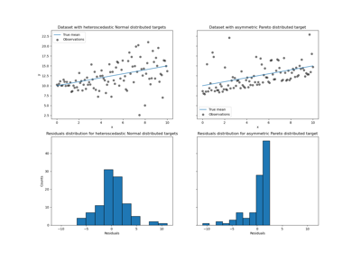
To make the problem interesting, we generate observations of the target y as the sum of a deterministic term computed by the function f and a random noise term that follows a centered log-normal. To make this even more interesting we consider the case where the amplitude of the noise depends on the input variable x (heteroscedastic noise).
The lognormal distribution is non-symmetric and long tailed: observing large outliers is likely but it is impossible to observe small outliers.
sigma = 0.5 + X.ravel() / 10
noise = rng.lognormal(sigma=sigma) - np.exp(sigma**2 / 2)
y = expected_y + noise
Split into train, test datasets:
X_train, X_test, y_train, y_test = train_test_split(X, y, random_state=0)
Fitting non-linear quantile and least squares regressors#
Fit gradient boosting models trained with the quantile loss and alpha=0.05,
alpha=0.5, alpha=0.95.
The models obtained for alpha=0.05 and alpha=0.95 produce a 90% coverage
interval (95% - 5% = 90%).
The model trained with alpha=0.5 produces a regression of the median: on
average, there should be the same number of target observations above and
below the predicted values.
from sklearn.ensemble import GradientBoostingRegressor
from sklearn.metrics import mean_pinball_loss, mean_squared_error

all_models = {}
common_params = dict(
    learning_rate=0.05,
    n_estimators=200,
    max_depth=2,
    min_samples_leaf=9,
    min_samples_split=9,
)
for alpha in [0.05, 0.5, 0.95]:
    gbr = GradientBoostingRegressor(loss="quantile", alpha=alpha, **common_params)
    all_models["q %1.2f" % alpha] = gbr.fit(X_train, y_train)
Notice that HistGradientBoostingRegressor is much
faster than GradientBoostingRegressor starting with
intermediate datasets (n_samples >= 10_000), which is not the case of the
present example.
For the sake of comparison, we also fit a baseline model trained with the usual (mean) squared error (MSE).
gbr_ls = GradientBoostingRegressor(loss="squared_error", **common_params)
all_models["mse"] = gbr_ls.fit(X_train, y_train)
Create an evenly spaced evaluation set of input values spanning the [0, 10] range.
x_plot = np.atleast_2d(np.linspace(0, 10, 1000)).T
Plot the true conditional mean function f, the predictions of the conditional mean (loss equals squared error), the conditional median and the conditional 90% interval (from 5th to 95th conditional percentiles).
import matplotlib.pyplot as plt

y_pred = all_models["mse"].predict(x_plot)
y_lower = all_models["q 0.05"].predict(x_plot)
y_upper = all_models["q 0.95"].predict(x_plot)
y_med = all_models["q 0.50"].predict(x_plot)

fig = plt.figure(figsize=(10, 10))
plt.plot(x_plot, f(x_plot), "black", linewidth=3, label=r"$f(x) = x\,\sin(x)$")
plt.plot(X_test, y_test, "b.", markersize=10, label="Test observations")
plt.plot(x_plot, y_med, "tab:orange", linewidth=3, label="Predicted median")
plt.plot(x_plot, y_pred, "tab:green", linewidth=3, label="Predicted mean")
plt.fill_between(
    x_plot.ravel(), y_lower, y_upper, alpha=0.4, label="Predicted 90% interval"
)
plt.xlabel("$x$")
plt.ylabel("$f(x)$")
plt.ylim(-10, 25)
plt.legend(loc="upper left")
plt.show()
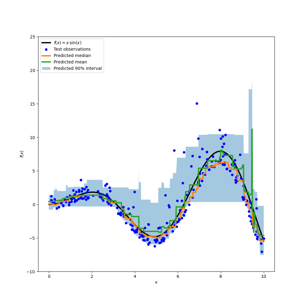
Comparing the predicted median with the predicted mean, we note that the median is on average below the mean as the noise is skewed towards high values (large outliers). The median estimate also seems to be smoother because of its natural robustness to outliers.
Also observe that the inductive bias of gradient boosting trees is unfortunately preventing our 0.05 quantile to fully capture the sinoisoidal shape of the signal, in particular around x=8. Tuning hyper-parameters can reduce this effect as shown in the last part of this notebook.
Analysis of the error metrics#
Measure the models with mean_squared_error and
mean_pinball_loss metrics on the training dataset.
import pandas as pd


def highlight_min(x):
    x_min = x.min()
    return ["font-weight: bold" if v == x_min else "" for v in x]


results = []
for name, gbr in sorted(all_models.items()):
    metrics = {"model": name}
    y_pred = gbr.predict(X_train)
    for alpha in [0.05, 0.5, 0.95]:
        metrics["pbl=%1.2f" % alpha] = mean_pinball_loss(y_train, y_pred, alpha=alpha)
    metrics["MSE"] = mean_squared_error(y_train, y_pred)
    results.append(metrics)

pd.DataFrame(results).set_index("model").style.apply(highlight_min)
One column shows all models evaluated by the same metric. The minimum number on a column should be obtained when the model is trained and measured with the same metric. This should be always the case on the training set if the training converged.
Note that because the target distribution is asymmetric, the expected conditional mean and conditional median are significantly different and therefore one could not use the squared error model get a good estimation of the conditional median nor the converse.
If the target distribution were symmetric and had no outliers (e.g. with a Gaussian noise), then median estimator and the least squares estimator would have yielded similar predictions.
We then do the same on the test set.
results = []
for name, gbr in sorted(all_models.items()):
    metrics = {"model": name}
    y_pred = gbr.predict(X_test)
    for alpha in [0.05, 0.5, 0.95]:
        metrics["pbl=%1.2f" % alpha] = mean_pinball_loss(y_test, y_pred, alpha=alpha)
    metrics["MSE"] = mean_squared_error(y_test, y_pred)
    results.append(metrics)

pd.DataFrame(results).set_index("model").style.apply(highlight_min)
Errors are higher meaning the models slightly overfitted the data. It still shows that the best test metric is obtained when the model is trained by minimizing this same metric.
Note that the conditional median estimator is competitive with the squared error estimator in terms of MSE on the test set: this can be explained by the fact the squared error estimator is very sensitive to large outliers which can cause significant overfitting. This can be seen on the right hand side of the previous plot. The conditional median estimator is biased (underestimation for this asymmetric noise) but is also naturally robust to outliers and overfits less.
Tuning the hyper-parameters of the quantile regressors#
In the plot above, we observed that the 5th percentile regressor seems to underfit and could not adapt to sinusoidal shape of the signal.
The hyper-parameters of the model were approximately hand-tuned for the median regressor and there is no reason that the same hyper-parameters are suitable for the 5th percentile regressor.
To confirm this hypothesis, we tune the hyper-parameters of a new regressor
of the 5th percentile by selecting the best model parameters by
cross-validation on the pinball loss with alpha=0.05:
from pprint import pprint

from sklearn.experimental import enable_halving_search_cv  # noqa: F401
from sklearn.metrics import make_scorer
from sklearn.model_selection import HalvingRandomSearchCV

param_grid = dict(
    learning_rate=[0.05, 0.1, 0.2],
    max_depth=[2, 5, 10],
    min_samples_leaf=[1, 5, 10, 20],
    min_samples_split=[5, 10, 20, 30, 50],
)
neg_mean_pinball_loss_05p_scorer = make_scorer(
    mean_pinball_loss,
    alpha=0.05,
    greater_is_better=False,  # maximize the negative loss
)
gbr = GradientBoostingRegressor(loss="quantile", alpha=0.05, random_state=0)
search_05p = HalvingRandomSearchCV(
    gbr,
    param_grid,
    resource="n_estimators",
    max_resources=250,
    min_resources=50,
    scoring=neg_mean_pinball_loss_05p_scorer,
    n_jobs=2,
    random_state=0,
).fit(X_train, y_train)
pprint(search_05p.best_params_)
{'learning_rate': 0.2,
 'max_depth': 2,
 'min_samples_leaf': 20,
 'min_samples_split': 10,
 'n_estimators': 150}
We observe that the hyper-parameters that were hand-tuned for the median regressor are in the same range as the hyper-parameters suitable for the 5th percentile regressor.
Let’s now tune the hyper-parameters for the 95th percentile regressor. We
need to redefine the scoring metric used to select the best model, along
with adjusting the alpha parameter of the inner gradient boosting estimator
itself:
from sklearn.base import clone

neg_mean_pinball_loss_95p_scorer = make_scorer(
    mean_pinball_loss,
    alpha=0.95,
    greater_is_better=False,  # maximize the negative loss
)
search_95p = clone(search_05p).set_params(
    estimator__alpha=0.95,
    scoring=neg_mean_pinball_loss_95p_scorer,
)
search_95p.fit(X_train, y_train)
pprint(search_95p.best_params_)
{'learning_rate': 0.05,
 'max_depth': 2,
 'min_samples_leaf': 5,
 'min_samples_split': 20,
 'n_estimators': 150}
The result shows that the hyper-parameters for the 95th percentile regressor identified by the search procedure are roughly in the same range as the hand-tuned hyper-parameters for the median regressor and the hyper-parameters identified by the search procedure for the 5th percentile regressor. However, the hyper-parameter searches did lead to an improved 90% coverage interval that is comprised by the predictions of those two tuned quantile regressors. Note that the prediction of the upper 95th percentile has a much coarser shape than the prediction of the lower 5th percentile because of the outliers:
y_lower_plot = search_05p.predict(x_plot)
y_upper_plot = search_95p.predict(x_plot)

fig = plt.figure(figsize=(10, 10))
plt.plot(x_plot, f(x_plot), "black", linewidth=3, label=r"$f(x) = x\,\sin(x)$")
plt.plot(X_test, y_test, "b.", markersize=10, label="Test observations")
plt.fill_between(
    x_plot.ravel(),
    y_lower_plot,
    y_upper_plot,
    alpha=0.4,
    label="Predicted 90% interval",
)
plt.xlabel("$x$")
plt.ylabel("$f(x)$")
plt.ylim(-10, 25)
plt.legend(loc="upper left")
plt.title("Prediction with tuned hyper-parameters")
plt.show()
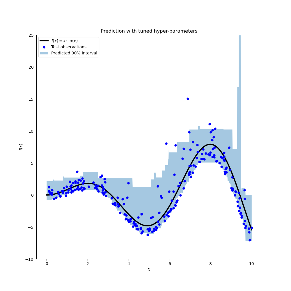
The plot looks qualitatively better than for the untuned models, especially for the shape of the of lower quantile.
Calibration of the confidence interval#
We can also evaluate the ability of the two extreme quantile estimators at
producing well-calibrated predictions of the 90%-coverage interval
(conditional on X), meaning that on average 90% of the observations should
lie within this interval.
To do this we can compute the coverage fraction, i.e. the proportion of observations that fall within the prediction intervals:
def coverage_fraction(y, y_low, y_high):
    return np.mean(np.logical_and(y >= y_low, y <= y_high))


coverage_fraction(y_train, search_05p.predict(X_train), search_95p.predict(X_train))
np.float64(0.9026666666666666)
On the training set the calibration is very close to the expected coverage value of 90%.
coverage_fraction(y_test, search_05p.predict(X_test), search_95p.predict(X_test))
np.float64(0.796)
On the test set, the estimated interval is too narrow to cover 90% of the test
points, but it may still hit the right coverage within reasonable statistical
uncertainty. We can use scipy.stats.bootstrap to measure the
variability of the coverage fraction at prediction time, without retraining
the models. We use a 95% confidence level for the estimated (bootstrapped)
interval of coverage; this is not to be confused with the 90% coverage
stemming from our 5% and 95% quantile predictions:
from scipy.stats import bootstrap

train_coverage_bs = bootstrap(
    (
        y_train,
        search_05p.predict(X_train),
        search_95p.predict(X_train),
    ),
    coverage_fraction,
    paired=True,
    confidence_level=0.95,
    n_resamples=1000,
)
ci = train_coverage_bs.confidence_interval
print(
    f"Training-set coverage lies between {ci.low:.1%} and {ci.high:.1%}, "
    f"based on a 95% bootstrap confidence interval."
)
Training-set coverage lies between 88.1% and 92.3%, based on a 95% bootstrap confidence interval.
Notice that the interval contains the target value of 90% coverage.
test_coverage_bs = bootstrap(
    (
        y_test,
        search_05p.predict(X_test),
        search_95p.predict(X_test),
    ),
    coverage_fraction,
    paired=True,
    confidence_level=0.95,
    n_resamples=1000,
)
ci = test_coverage_bs.confidence_interval
print(
    f"Test-set coverage lies between {ci.low:.1%} and {ci.high:.1%}, "
    f"based on a 95% bootstrap confidence interval."
)
Test-set coverage lies between 73.8% and 84.4%, based on a 95% bootstrap confidence interval.
The quantile estimates from the tuned models are sadly not well-calibrated on the test set: the width of the estimated confidence interval is too narrow even when taking it’s variations into account.
Total running time of the script: (0 minutes 13.266 seconds)
Related examples

Gaussian Processes regression: basic introductory example