Note
Go to the end to download the full example code or to run this example in your browser via JupyterLite or Binder.
Semi-supervised Classification on a Text Dataset#
This example demonstrates the effectiveness of semi-supervised learning
for text classification on TF-IDF features when labeled data
is scarce. For such purpose we compare four different approaches:
Supervised learning using 100% of labels in the training set (best-case scenario)
Uses
SGDClassifierwith full supervisionRepresents the best possible performance when labeled data is abundant
Supervised learning using 20% of labels in the training set (baseline)
Same model as the best-case scenario but trained on a random 20% subset of the labeled training data
Shows the performance degradation of a fully supervised model due to limited labeled data
SelfTrainingClassifier(semi-supervised)Uses 20% labeled data + 80% unlabeled data for training
Iteratively predicts labels for unlabeled data
Demonstrates how self-training can improve performance
LabelSpreading(semi-supervised)Uses 20% labeled data + 80% unlabeled data for training
Propagates labels through the data manifold
Shows how graph-based methods can leverage unlabeled data
The example uses the 20 newsgroups dataset, focusing on five categories. The results demonstrate how semi-supervised methods can achieve better performance than supervised learning with limited labeled data by effectively utilizing unlabeled samples.
# Authors: The scikit-learn developers
# SPDX-License-Identifier: BSD-3-Clause
from sklearn.datasets import fetch_20newsgroups
from sklearn.feature_extraction.text import CountVectorizer, TfidfTransformer
from sklearn.linear_model import SGDClassifier
from sklearn.metrics import f1_score
from sklearn.model_selection import train_test_split
from sklearn.pipeline import Pipeline
from sklearn.semi_supervised import LabelSpreading, SelfTrainingClassifier

# Loading dataset containing first five categories
data = fetch_20newsgroups(
    subset="train",
    categories=[
        "alt.atheism",
        "comp.graphics",
        "comp.os.ms-windows.misc",
        "comp.sys.ibm.pc.hardware",
        "comp.sys.mac.hardware",
    ],
)

# Parameters
sdg_params = dict(alpha=1e-5, penalty="l2", loss="log_loss")
vectorizer_params = dict(ngram_range=(1, 2), min_df=5, max_df=0.8)

# Supervised Pipeline
pipeline = Pipeline(
    [
        ("vect", CountVectorizer(**vectorizer_params)),
        ("tfidf", TfidfTransformer()),
        ("clf", SGDClassifier(**sdg_params)),
    ]
)
# SelfTraining Pipeline
st_pipeline = Pipeline(
    [
        ("vect", CountVectorizer(**vectorizer_params)),
        ("tfidf", TfidfTransformer()),
        ("clf", SelfTrainingClassifier(SGDClassifier(**sdg_params))),
    ]
)
# LabelSpreading Pipeline
ls_pipeline = Pipeline(
    [
        ("vect", CountVectorizer(**vectorizer_params)),
        ("tfidf", TfidfTransformer()),
        ("clf", LabelSpreading()),
    ]
)


def eval_and_get_f1(clf, X_train, y_train, X_test, y_test):
    """Evaluate model performance and return F1 score"""
    print(f"   Number of training samples: {len(X_train)}")
    print(f"   Unlabeled samples in training set: {sum(1 for x in y_train if x == -1)}")
    clf.fit(X_train, y_train)
    y_pred = clf.predict(X_test)
    f1 = f1_score(y_test, y_pred, average="micro")
    print(f"   Micro-averaged F1 score on test set: {f1:.3f}")
    print("\n")
    return f1


X, y = data.data, data.target
X_train, X_test, y_train, y_test = train_test_split(X, y)
1. Evaluate a supervised SGDClassifier using 100% of the (labeled) training set. This represents the best-case performance when the model has full access to all labeled examples.
f1_scores = {}
print("1. Supervised SGDClassifier on 100% of the data:")
f1_scores["Supervised (100%)"] = eval_and_get_f1(
    pipeline, X_train, y_train, X_test, y_test
)
1. Supervised SGDClassifier on 100% of the data:
   Number of training samples: 2117
   Unlabeled samples in training set: 0
   Micro-averaged F1 score on test set: 0.901
2. Evaluate a supervised SGDClassifier trained on only 20% of the data. This serves as a baseline to illustrate the performance drop caused by limiting the training samples.
import numpy as np

print("2. Supervised SGDClassifier on 20% of the training data:")
rng = np.random.default_rng(42)
y_mask = rng.random(len(y_train)) < 0.2
# X_20 and y_20 are the subset of the train dataset indicated by the mask
X_20, y_20 = map(list, zip(*((x, y) for x, y, m in zip(X_train, y_train, y_mask) if m)))
f1_scores["Supervised (20%)"] = eval_and_get_f1(pipeline, X_20, y_20, X_test, y_test)
2. Supervised SGDClassifier on 20% of the training data:
   Number of training samples: 434
   Unlabeled samples in training set: 0
   Micro-averaged F1 score on test set: 0.775
3. Evaluate a semi-supervised SelfTrainingClassifier using 20% labeled and 80% unlabeled data. The remaining 80% of the training labels are masked as unlabeled (-1), allowing the model to iteratively label and learn from them.
print(
    "3. SelfTrainingClassifier (semi-supervised) using 20% labeled "
    "+ 80% unlabeled data):"
)
y_train_semi = y_train.copy()
y_train_semi[~y_mask] = -1
f1_scores["SelfTraining"] = eval_and_get_f1(
    st_pipeline, X_train, y_train_semi, X_test, y_test
)
3. SelfTrainingClassifier (semi-supervised) using 20% labeled + 80% unlabeled data):
   Number of training samples: 2117
   Unlabeled samples in training set: 1683
   Micro-averaged F1 score on test set: 0.829
4. Evaluate a semi-supervised LabelSpreading model using 20% labeled and 80% unlabeled data. Like SelfTraining, the model infers labels for the unlabeled portion of the data to enhance performance.
print("4. LabelSpreading (semi-supervised) using 20% labeled + 80% unlabeled data:")
f1_scores["LabelSpreading"] = eval_and_get_f1(
    ls_pipeline, X_train, y_train_semi, X_test, y_test
)
4. LabelSpreading (semi-supervised) using 20% labeled + 80% unlabeled data:
   Number of training samples: 2117
   Unlabeled samples in training set: 1683
   Micro-averaged F1 score on test set: 0.647
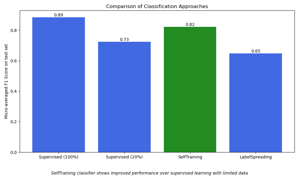
Plot results#
Visualize the performance of different classification approaches using a bar chart.
This helps to compare how each method performs based on the
micro-averaged f1_score.
Micro-averaging computes metrics globally across all classes,
which gives a single overall measure of performance and allows fair comparison
between the different approaches, even in the presence of class imbalance.
import matplotlib.pyplot as plt

plt.figure(figsize=(10, 6))

models = list(f1_scores.keys())
scores = list(f1_scores.values())

colors = ["royalblue", "royalblue", "forestgreen", "royalblue"]
bars = plt.bar(models, scores, color=colors)

plt.title("Comparison of Classification Approaches")
plt.ylabel("Micro-averaged F1 Score on test set")
plt.xticks()

for bar in bars:
    height = bar.get_height()
    plt.text(
        bar.get_x() + bar.get_width() / 2.0,
        height,
        f"{height:.2f}",
        ha="center",
        va="bottom",
    )

plt.figtext(
    0.5,
    0.02,
    "SelfTraining classifier shows improved performance over "
    "supervised learning with limited data",
    ha="center",
    va="bottom",
    fontsize=10,
    style="italic",
)

plt.tight_layout()
plt.subplots_adjust(bottom=0.15)
plt.show()
Total running time of the script: (0 minutes 6.210 seconds)
Related examples
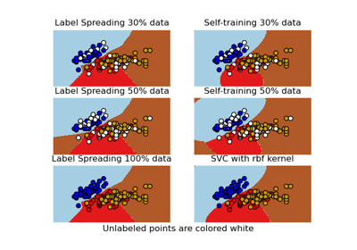
Decision boundary of semi-supervised classifiers versus SVM on the Iris dataset
Label Propagation digits: Demonstrating performance