Note

Go to the end to download the full example code or to run this example in your browser via JupyterLite or Binder.

Probability Calibration curves#

When performing classification one often wants to predict not only the class label, but also the associated probability. This probability gives some kind of confidence on the prediction. This example demonstrates how to visualize how well calibrated the predicted probabilities are using calibration curves, also known as reliability diagrams. Calibration of an uncalibrated classifier will also be demonstrated.

# Authors: The scikit-learn developers
# SPDX-License-Identifier: BSD-3-Clause

Dataset#

We use a synthetic binary classification dataset with 100,000 samples and 20 features. Of the 20 features, only 2 are informative, 10 are redundant (random combinations of the informative features) and the remaining 8 are uninformative (random numbers). Of the 100,000 samples, 1,000 will be used for model fitting (possibly shared with post-hoc calibration) and the rest for evaluation.

from sklearn.datasets import make_classification
from sklearn.model_selection import train_test_split

n_samples_total = 100_000
n_samples_train = 1_000

X, y = make_classification(
    n_samples=n_samples_total,
    n_features=20,
    n_informative=2,
    n_redundant=10,
    weights=[0.666, 0.333],
    n_clusters_per_class=2,
    random_state=42,
)
X_train, X_test, y_train, y_test = train_test_split(
    X, y, train_size=n_samples_train, random_state=42
)

Calibration curves#

Gaussian Naive Bayes#

First, we will compare:

LogisticRegressionCV (used as baseline since very often, properly regularized logistic regression is well calibrated by default thanks to the use of the log-loss)
Uncalibrated GaussianNB
GaussianNB with isotonic and sigmoid calibration (see User Guide)

Calibration curves for all 4 conditions are plotted below, with the average predicted probability for each bin on the x-axis and the fraction of positive classes in each bin on the y-axis.

import matplotlib.pyplot as plt
from matplotlib.gridspec import GridSpec

from sklearn.calibration import CalibratedClassifierCV, CalibrationDisplay
from sklearn.linear_model import LogisticRegressionCV
from sklearn.naive_bayes import GaussianNB

lr = LogisticRegressionCV(
    Cs=10, scoring="neg_log_loss", l1_ratios=(0,), use_legacy_attributes=False
)
gnb = GaussianNB()
gnb_isotonic = CalibratedClassifierCV(gnb, cv=10, method="isotonic")
gnb_sigmoid = CalibratedClassifierCV(gnb, cv=10, method="sigmoid")

clf_list = [
    (lr, "Logistic"),
    (gnb, "Naive Bayes"),
    (gnb_isotonic, "Naive Bayes + Isotonic"),
    (gnb_sigmoid, "Naive Bayes + Sigmoid"),
]

fig = plt.figure(figsize=(10, 10))
gs = GridSpec(4, 2)
colors = plt.get_cmap("Dark2")

ax_calibration_curve = fig.add_subplot(gs[:2, :2])
calibration_displays = {}
for i, (clf, name) in enumerate(clf_list):
    clf.fit(X_train, y_train)
    display = CalibrationDisplay.from_estimator(
        clf,
        X_test,
        y_test,
        n_bins=10,
        strategy="quantile",
        name=name,
        ax=ax_calibration_curve,
        color=colors(i),
    )
    calibration_displays[name] = display

ax_calibration_curve.grid()
ax_calibration_curve.set_title("Calibration plots (Naive Bayes)")

# Add histogram
grid_positions = [(2, 0), (2, 1), (3, 0), (3, 1)]
for i, (_, name) in enumerate(clf_list):
    row, col = grid_positions[i]
    ax = fig.add_subplot(gs[row, col])

    ax.hist(
        calibration_displays[name].y_prob,
        range=(0, 1),
        bins=10,
        label=name,
        color=colors(i),
    )
    ax.set(title=name, xlabel="Mean predicted probability", ylabel="Count")

plt.tight_layout()
plt.show()

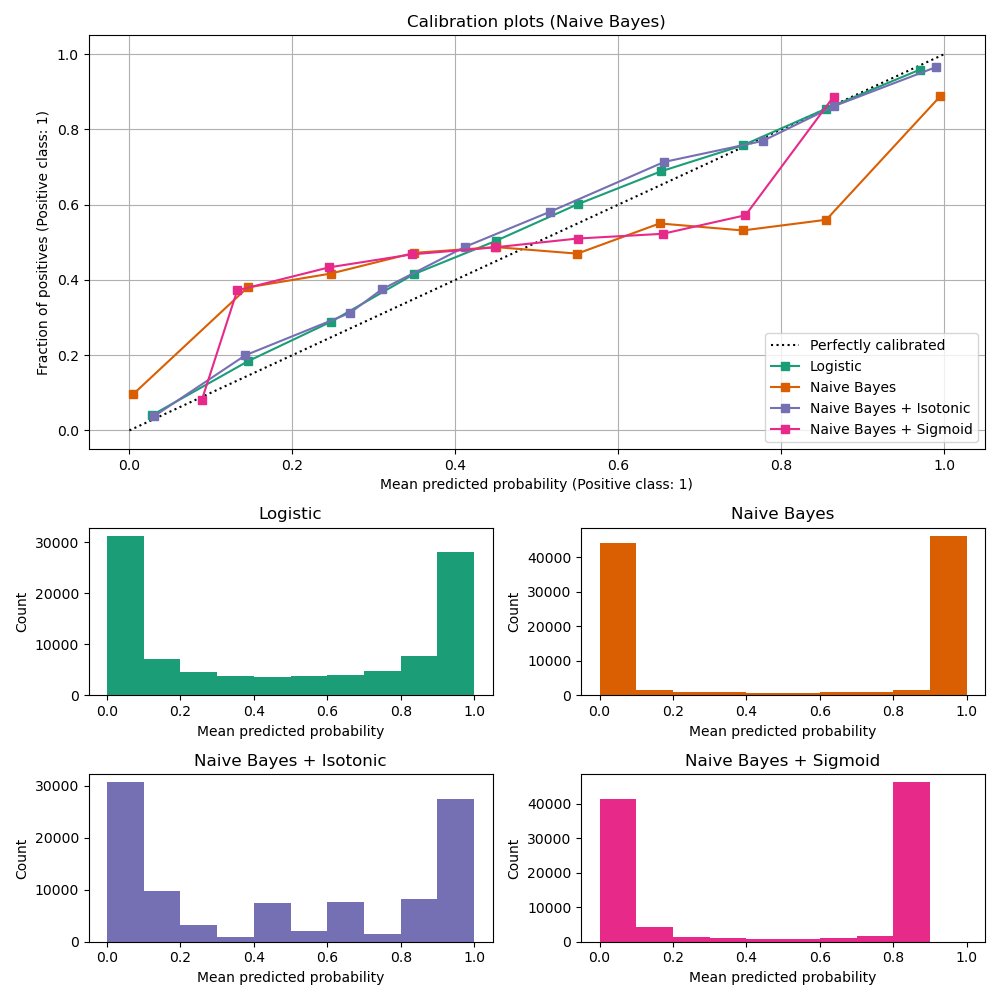
Calibration plots (Naive Bayes), Logistic, Naive Bayes, Naive Bayes + Isotonic, Naive Bayes + Sigmoid

The logistic regression classifier is well calibrated by default, as indicated by the diagonal calibration curve. This is not surprising since we adjusted the regularization parameter to minimize the Log loss via internal cross-validation.

On the contrary GaussianNB is poorly calibrated because of the redundant features which violate the assumption of feature-independence. It results in an overly confident classifier, which is indicated by the typical transposed-sigmoid calibration curve.

Post-hoc calibration of the predicted probabilities of GaussianNB with Isotonic regression or Sigmoid regression fix this issue to a good extent as can be seen from the nearly diagonal calibration curve. Neither method is perfect because of the limited amount of training and calibration data (1,000 samples for both).

Below we make a quantitative analysis considering several classification metrics: Brier score loss, Log loss, precision, recall, F1 score and ROC AUC.

from collections import defaultdict

import pandas as pd

from sklearn.metrics import (
    brier_score_loss,
    f1_score,
    log_loss,
    precision_score,
    recall_score,
    roc_auc_score,
)


def compute_metrics(clf_list, X_train, y_train, X_test, y_test):
    scores = defaultdict(list)
    for i, (clf, name) in enumerate(clf_list):
        clf.fit(X_train, y_train)
        y_prob = clf.predict_proba(X_test)
        y_pred = clf.predict(X_test)
        scores["Classifier"].append(name)

        for metric in [brier_score_loss, log_loss, roc_auc_score]:
            score_name = (
                metric.__name__.replace("_", " ").replace("score", "").capitalize()
            )
            scores[score_name].append(metric(y_test, y_prob[:, 1]))

        for metric in [precision_score, recall_score, f1_score]:
            score_name = (
                metric.__name__.replace("_", " ").replace("score", "").capitalize()
            )
            scores[score_name].append(metric(y_test, y_pred))

    score_df = pd.DataFrame(scores).set_index("Classifier")
    return score_df.round(decimals=3)


compute_metrics(clf_list, X_train, y_train, X_test, y_test)

	Brier loss	Log loss	Roc auc	Precision	Recall	F1
Classifier
Logistic	0.090	0.296	0.938	0.841	0.776	0.807
Naive Bayes	0.115	0.774	0.940	0.773	0.857	0.813
Naive Bayes + Isotonic	0.091	0.340	0.939	0.842	0.778	0.808
Naive Bayes + Sigmoid	0.090	0.294	0.940	0.849	0.764	0.804

Post-hoc calibration improves the Brier score loss and Log loss. Both metrics can be decomposed into calibration and refinement terms and are thus sensitive to the calibration of the predicted probabilities.

The ROC AUC score is a pure ranking metric. It is not changed by a strictly monotonic transformation of the predicted probabilities, like the sigmoid calibration. However, the isotonic calibration method can degrade the ROC AUC score a bit because it is not a strictly monotonic transformation, only a monotonic one (constant piecewise transformation).

Post-hoc calibration can significantly alter metrics computed on discrete predictions such as precision, recall and F1 score. This is because calibration change prediction probabilities at the location of the default decision threshold (at x = 0.5 on the graph), especially when the classification problem is not balanced. FixedThresholder and TunedThresholdClassifierCV can help assess the impact of different decision thresholds on the value of F1 score.

Linear support vector classifier#

Next, we will compare:

LogisticRegressionCV (baseline)
Uncalibrated LinearSVC. Since support vector machines do not output probabilities by default, we naively scale the output of the decision_function into [0, 1] by applying min-max scaling.
LinearSVC with isotonic and sigmoid calibration (see User Guide)

import numpy as np

from sklearn.svm import LinearSVC


class NaivelyCalibratedLinearSVC(LinearSVC):
    """LinearSVC with `predict_proba` method that naively scales
    `decision_function` output for binary classification."""

    def fit(self, X, y):
        super().fit(X, y)
        df = self.decision_function(X)
        self.df_min_ = df.min()
        self.df_max_ = df.max()

    def predict_proba(self, X):
        """Min-max scale output of `decision_function` to [0, 1]."""
        df = self.decision_function(X)
        calibrated_df = (df - self.df_min_) / (self.df_max_ - self.df_min_)
        proba_pos_class = np.clip(calibrated_df, 0, 1)
        proba_neg_class = 1 - proba_pos_class
        proba = np.c_[proba_neg_class, proba_pos_class]
        return proba

svc = NaivelyCalibratedLinearSVC(max_iter=10_000)
svc_isotonic = CalibratedClassifierCV(svc, cv=2, method="isotonic")
svc_sigmoid = CalibratedClassifierCV(svc, cv=2, method="sigmoid")

clf_list = [
    (lr, "Logistic"),
    (svc, "SVC"),
    (svc_isotonic, "SVC + Isotonic"),
    (svc_sigmoid, "SVC + Sigmoid"),
]

fig = plt.figure(figsize=(10, 10))
gs = GridSpec(4, 2)

ax_calibration_curve = fig.add_subplot(gs[:2, :2])
calibration_displays = {}
for i, (clf, name) in enumerate(clf_list):
    clf.fit(X_train, y_train)
    display = CalibrationDisplay.from_estimator(
        clf,
        X_test,
        y_test,
        n_bins=10,
        name=name,
        strategy="quantile",
        ax=ax_calibration_curve,
        color=colors(i),
    )
    calibration_displays[name] = display

ax_calibration_curve.grid()
ax_calibration_curve.set_title("Calibration plots (SVC)")

# Add histogram
grid_positions = [(2, 0), (2, 1), (3, 0), (3, 1)]
for i, (_, name) in enumerate(clf_list):
    row, col = grid_positions[i]
    ax = fig.add_subplot(gs[row, col])

    ax.hist(
        calibration_displays[name].y_prob,
        range=(0, 1),
        bins=10,
        label=name,
        color=colors(i),
    )
    ax.set(title=name, xlabel="Mean predicted probability", ylabel="Count")

plt.tight_layout()
plt.show()

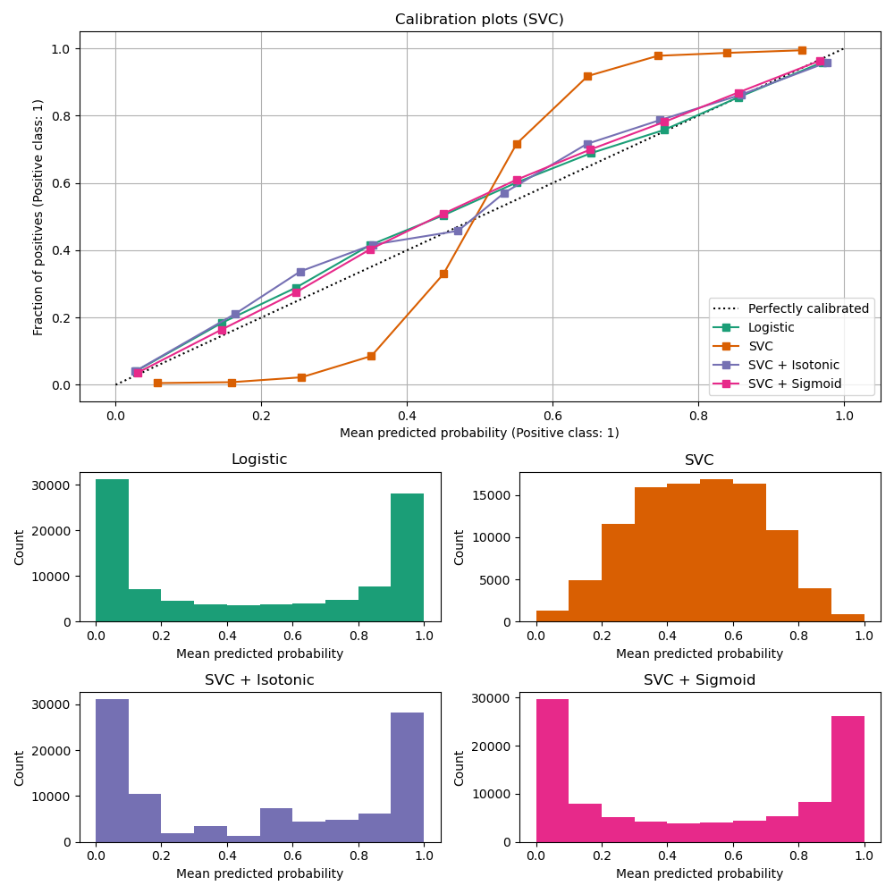
Calibration plots (SVC), Logistic, SVC, SVC + Isotonic, SVC + Sigmoid

The raw LinearSVC classifier shows the opposite behavior to GaussianNB; the calibration curve has a sigmoid shape, which is typical for an under-confident classifier. In the case of LinearSVC, this is caused by the margin property of the hinge loss, which focuses on samples that are close to the decision boundary (support vectors). Samples that are far away from the decision boundary do not impact the hinge loss. It thus makes sense that LinearSVC does not try to separate samples in the high confidence region regions. This leads to flatter calibration curves near 0 and 1 and is empirically shown with a variety of datasets in Niculescu-Mizil & Caruana [1].

Both kinds of calibration (sigmoid and isotonic) can fix this issue and yield similar results.

As before, we show the Brier score loss, Log loss, precision, recall, F1 score and ROC AUC.

compute_metrics(clf_list, X_train, y_train, X_test, y_test)

	Brier loss	Log loss	Roc auc	Precision	Recall	F1
Classifier
Logistic	0.090	0.296	0.938	0.841	0.776	0.807
SVC	0.142	0.458	0.938	0.834	0.782	0.807
SVC + Isotonic	0.092	0.376	0.936	0.826	0.792	0.809
SVC + Sigmoid	0.091	0.299	0.938	0.842	0.770	0.805

As with GaussianNB above, calibration improves both Brier score loss and Log loss. ROC AUC is not affected by the sigmoid calibration and slightly degraded by isotonic calibration for the same reason as above.

Again, metrics computed on thresholded predictions (e.g. such as precision, recall and F1 score) can be impacted because thresholding the predicted probabilities at 0.5 has a different effect before and after calibration.

Summary#

Parametric sigmoid calibration can deal with situations where the calibration curve of the base classifier is sigmoid (e.g. the underconfident LinearSVC) or transposed-sigmoid (e.g. the overconfident GaussianNB). Non-parametric isotonic calibration can also fix the calibration problem but may require more data to produce good results.