Note
Go to the end to download the full example code or to run this example in your browser via JupyterLite or Binder.
Release Highlights for scikit-learn 1.4#
We are pleased to announce the release of scikit-learn 1.4! Many bug fixes and improvements were added, as well as some new key features. We detail below a few of the major features of this release. For an exhaustive list of all the changes, please refer to the release notes.
To install the latest version (with pip):
pip install --upgrade scikit-learn
or with conda:
conda install -c conda-forge scikit-learn
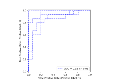
HistGradientBoosting Natively Supports Categorical DTypes in DataFrames#
ensemble.HistGradientBoostingClassifier and
ensemble.HistGradientBoostingRegressor now directly supports dataframes with
categorical features. Here we have a dataset with a mixture of
categorical and numerical features:
from sklearn.datasets import fetch_openml

X_adult, y_adult = fetch_openml("adult", version=2, return_X_y=True)

# Remove redundant and non-feature columns
X_adult = X_adult.drop(["education-num", "fnlwgt"], axis="columns")
X_adult.dtypes
age                  int64
workclass         category
education         category
marital-status    category
occupation        category
relationship      category
race              category
sex               category
capital-gain         int64
capital-loss         int64
hours-per-week       int64
native-country    category
dtype: object
By setting categorical_features="from_dtype", the gradient boosting classifier
treats the columns with categorical dtypes as categorical features in the
algorithm:
from sklearn.ensemble import HistGradientBoostingClassifier
from sklearn.metrics import roc_auc_score
from sklearn.model_selection import train_test_split

X_train, X_test, y_train, y_test = train_test_split(X_adult, y_adult, random_state=0)
hist = HistGradientBoostingClassifier(categorical_features="from_dtype")

hist.fit(X_train, y_train)
y_decision = hist.decision_function(X_test)
print(f"ROC AUC score is {roc_auc_score(y_test, y_decision)}")
ROC AUC score is 0.9284706281446747
Polars output in set_output#
scikit-learn’s transformers now support polars output with the set_output API.
import polars as pl

from sklearn.compose import ColumnTransformer
from sklearn.preprocessing import OneHotEncoder, StandardScaler

df = pl.DataFrame(
    {"height": [120, 140, 150, 110, 100], "pet": ["dog", "cat", "dog", "cat", "cat"]}
)
preprocessor = ColumnTransformer(
    [
        ("numerical", StandardScaler(), ["height"]),
        ("categorical", OneHotEncoder(sparse_output=False), ["pet"]),
    ],
    verbose_feature_names_out=False,
)
preprocessor.set_output(transform="polars")

df_out = preprocessor.fit_transform(df)
df_out
print(f"Output type: {type(df_out)}")
Output type: <class 'polars.dataframe.frame.DataFrame'>
Missing value support for Random Forest#
The classes ensemble.RandomForestClassifier and
ensemble.RandomForestRegressor now support missing values. When training
every individual tree, the splitter evaluates each potential threshold with the
missing values going to the left and right nodes. More details in the
User Guide.
import numpy as np

from sklearn.ensemble import RandomForestClassifier

X = np.array([0, 1, 6, np.nan]).reshape(-1, 1)
y = [0, 0, 1, 1]

forest = RandomForestClassifier(random_state=0).fit(X, y)
forest.predict(X)
array([0, 0, 1, 1])
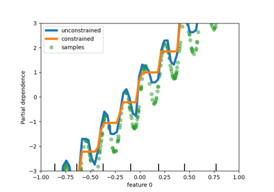
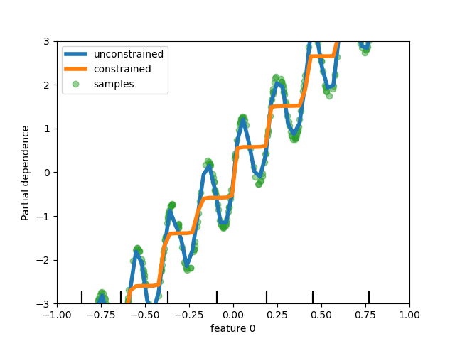
Add support for monotonic constraints in tree-based models#
While we added support for monotonic constraints in histogram-based gradient boosting in scikit-learn 0.23, we now support this feature for all other tree-based models as trees, random forests, extra-trees, and exact gradient boosting. Here, we show this feature for random forest on a regression problem.
import matplotlib.pyplot as plt

from sklearn.ensemble import RandomForestRegressor
from sklearn.inspection import PartialDependenceDisplay

n_samples = 500
rng = np.random.RandomState(0)
X = rng.randn(n_samples, 2)
noise = rng.normal(loc=0.0, scale=0.01, size=n_samples)
y = 5 * X[:, 0] + np.sin(10 * np.pi * X[:, 0]) - noise

rf_no_cst = RandomForestRegressor().fit(X, y)
rf_cst = RandomForestRegressor(monotonic_cst=[1, 0]).fit(X, y)

disp = PartialDependenceDisplay.from_estimator(
    rf_no_cst,
    X,
    features=[0],
    feature_names=["feature 0"],
    line_kw={"linewidth": 4, "label": "unconstrained", "color": "tab:blue"},
)
PartialDependenceDisplay.from_estimator(
    rf_cst,
    X,
    features=[0],
    line_kw={"linewidth": 4, "label": "constrained", "color": "tab:orange"},
    ax=disp.axes_,
)
disp.axes_[0, 0].plot(
    X[:, 0], y, "o", alpha=0.5, zorder=-1, label="samples", color="tab:green"
)
disp.axes_[0, 0].set_ylim(-3, 3)
disp.axes_[0, 0].set_xlim(-1, 1)
disp.axes_[0, 0].legend()
plt.show()
Enriched estimator displays#
Estimators displays have been enriched: if we look at forest, defined above:
forest
One can access the documentation of the estimator by clicking on the icon “?” on the top right corner of the diagram.
In addition, the display changes color, from orange to blue, when the estimator is fitted. You can also get this information by hovering on the icon “i”.
from sklearn.base import clone

clone(forest)  # the clone is not fitted
Metadata Routing Support#
Many meta-estimators and cross-validation routines now support metadata
routing, which are listed in the user guide. For instance, this is how you can do a nested
cross-validation with sample weights and GroupKFold:
import sklearn
from sklearn.datasets import make_regression
from sklearn.linear_model import Lasso
from sklearn.metrics import get_scorer
from sklearn.model_selection import GridSearchCV, GroupKFold, cross_validate

# For now by default metadata routing is disabled, and need to be explicitly
# enabled.
sklearn.set_config(enable_metadata_routing=True)

n_samples = 100
X, y = make_regression(n_samples=n_samples, n_features=5, noise=0.5)
rng = np.random.RandomState(7)
groups = rng.randint(0, 10, size=n_samples)
sample_weights = rng.rand(n_samples)
estimator = Lasso().set_fit_request(sample_weight=True)
hyperparameter_grid = {"alpha": [0.1, 0.5, 1.0, 2.0]}
scoring_inner_cv = get_scorer("neg_mean_squared_error").set_score_request(
    sample_weight=True
)
inner_cv = GroupKFold(n_splits=5)

grid_search = GridSearchCV(
    estimator=estimator,
    param_grid=hyperparameter_grid,
    cv=inner_cv,
    scoring=scoring_inner_cv,
)

outer_cv = GroupKFold(n_splits=5)
scorers = {
    "mse": get_scorer("neg_mean_squared_error").set_score_request(sample_weight=True)
}
results = cross_validate(
    grid_search,
    X,
    y,
    cv=outer_cv,
    scoring=scorers,
    return_estimator=True,
    params={"sample_weight": sample_weights, "groups": groups},
)
print("cv error on test sets:", results["test_mse"])

# Setting the flag to the default `False` to avoid interference with other
# scripts.
sklearn.set_config(enable_metadata_routing=False)
cv error on test sets: [-0.12854109 -0.44508726 -0.25848332 -0.29688232 -0.15773258]
Improved memory and runtime efficiency for PCA on sparse data#
PCA is now able to handle sparse matrices natively for the arpack
solver by levaraging scipy.sparse.linalg.LinearOperator to avoid
materializing large sparse matrices when performing the
eigenvalue decomposition of the data set covariance matrix.
from time import time

import scipy.sparse as sp

from sklearn.decomposition import PCA

X_sparse = sp.random(m=1000, n=1000, random_state=0)
X_dense = X_sparse.toarray()

t0 = time()
PCA(n_components=10, svd_solver="arpack").fit(X_sparse)
time_sparse = time() - t0

t0 = time()
PCA(n_components=10, svd_solver="arpack").fit(X_dense)
time_dense = time() - t0

print(f"Speedup: {time_dense / time_sparse:.1f}x")
Speedup: 4.2x
Total running time of the script: (0 minutes 2.022 seconds)
Related examples