Note
Go to the end to download the full example code or to run this example in your browser via JupyterLite or Binder.
Compare cross decomposition methods#
Simple usage of various cross decomposition algorithms:
PLSCanonical
PLSRegression, with multivariate response, a.k.a. PLS2
PLSRegression, with univariate response, a.k.a. PLS1
CCA
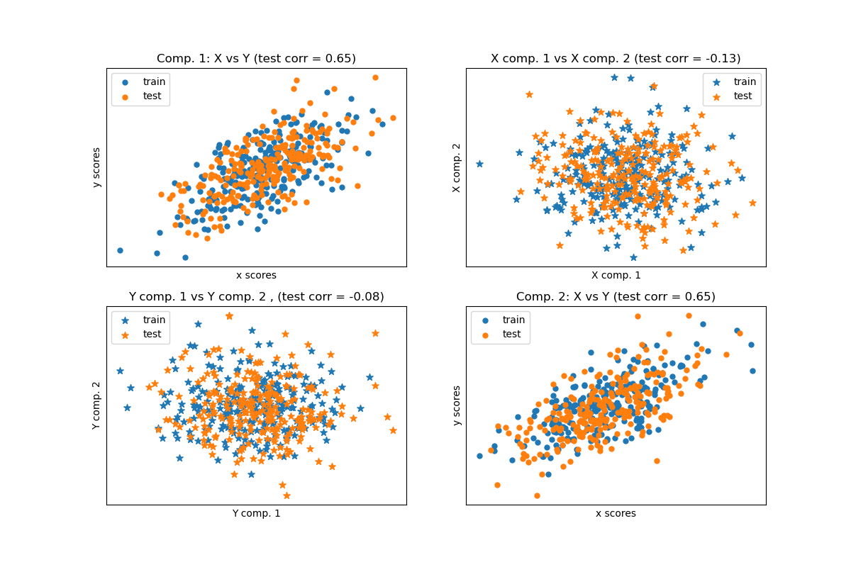
Given 2 multivariate covarying two-dimensional datasets, X, and Y, PLS extracts the ‘directions of covariance’, i.e. the components of each datasets that explain the most shared variance between both datasets. This is apparent on the scatterplot matrix display: components 1 in dataset X and dataset Y are maximally correlated (points lie around the first diagonal). This is also true for components 2 in both dataset, however, the correlation across datasets for different components is weak: the point cloud is very spherical.
# Authors: The scikit-learn developers
# SPDX-License-Identifier: BSD-3-Clause
Dataset based latent variables model#
import numpy as np

from sklearn.model_selection import train_test_split

rng = np.random.default_rng(42)

n = 500
# 2 latents vars:
l1 = rng.normal(size=n)
l2 = rng.normal(size=n)

latents = np.array([l1, l1, l2, l2]).T
X = latents + rng.normal(size=(n, 4))
Y = latents + rng.normal(size=(n, 4))

X_train, X_test, Y_train, Y_test = train_test_split(X, Y, test_size=0.5, shuffle=False)

print("Corr(X)")
print(np.round(np.corrcoef(X.T), 2))
print("Corr(Y)")
print(np.round(np.corrcoef(Y.T), 2))
Corr(X)
[[ 1.    0.48 -0.01  0.  ]
 [ 0.48  1.   -0.01  0.  ]
 [-0.01 -0.01  1.    0.49]
 [ 0.    0.    0.49  1.  ]]
Corr(Y)
[[ 1.    0.47  0.03  0.05]
 [ 0.47  1.    0.03 -0.01]
 [ 0.03  0.03  1.    0.5 ]
 [ 0.05 -0.01  0.5   1.  ]]
Canonical (symmetric) PLS#
Transform data#
from sklearn.cross_decomposition import PLSCanonical

plsca = PLSCanonical(n_components=2)
plsca.fit(X_train, Y_train)
X_train_r, Y_train_r = plsca.transform(X_train, Y_train)
X_test_r, Y_test_r = plsca.transform(X_test, Y_test)
Scatter plot of scores#
import matplotlib.pyplot as plt

# On diagonal plot X vs Y scores on each components
plt.figure(figsize=(12, 8))
plt.subplot(221)
plt.scatter(X_train_r[:, 0], Y_train_r[:, 0], label="train", marker="o", s=25)
plt.scatter(X_test_r[:, 0], Y_test_r[:, 0], label="test", marker="o", s=25)
plt.xlabel("x scores")
plt.ylabel("y scores")
plt.title(
    "Comp. 1: X vs Y (test corr = %.2f)"
    % np.corrcoef(X_test_r[:, 0], Y_test_r[:, 0])[0, 1]
)
plt.xticks(())
plt.yticks(())
plt.legend(loc="best")

plt.subplot(224)
plt.scatter(X_train_r[:, 1], Y_train_r[:, 1], label="train", marker="o", s=25)
plt.scatter(X_test_r[:, 1], Y_test_r[:, 1], label="test", marker="o", s=25)
plt.xlabel("x scores")
plt.ylabel("y scores")
plt.title(
    "Comp. 2: X vs Y (test corr = %.2f)"
    % np.corrcoef(X_test_r[:, 1], Y_test_r[:, 1])[0, 1]
)
plt.xticks(())
plt.yticks(())
plt.legend(loc="best")

# Off diagonal plot components 1 vs 2 for X and Y
plt.subplot(222)
plt.scatter(X_train_r[:, 0], X_train_r[:, 1], label="train", marker="*", s=50)
plt.scatter(X_test_r[:, 0], X_test_r[:, 1], label="test", marker="*", s=50)
plt.xlabel("X comp. 1")
plt.ylabel("X comp. 2")
plt.title(
    "X comp. 1 vs X comp. 2 (test corr = %.2f)"
    % np.corrcoef(X_test_r[:, 0], X_test_r[:, 1])[0, 1]
)
plt.legend(loc="best")
plt.xticks(())
plt.yticks(())

plt.subplot(223)
plt.scatter(Y_train_r[:, 0], Y_train_r[:, 1], label="train", marker="*", s=50)
plt.scatter(Y_test_r[:, 0], Y_test_r[:, 1], label="test", marker="*", s=50)
plt.xlabel("Y comp. 1")
plt.ylabel("Y comp. 2")
plt.title(
    "Y comp. 1 vs Y comp. 2 , (test corr = %.2f)"
    % np.corrcoef(Y_test_r[:, 0], Y_test_r[:, 1])[0, 1]
)
plt.legend(loc="best")
plt.xticks(())
plt.yticks(())
plt.show()
PLS regression, with multivariate response, a.k.a. PLS2#
from sklearn.cross_decomposition import PLSRegression

n = 1000
q = 3
p = 10
X = rng.normal(size=(n, p))
B = np.array([[1, 2] + [0] * (p - 2)] * q).T
# each Yj = 1*X1 + 2*X2 + noize
Y = np.dot(X, B) + rng.normal(size=(n, q)) + 5

pls2 = PLSRegression(n_components=3)
pls2.fit(X, Y)
print("True B (such that: Y = XB + Err)")
print(B)
# compare pls2.coef_ with B
print("Estimated B")
print(np.round(pls2.coef_, 1))
pls2.predict(X)
True B (such that: Y = XB + Err)
[[1 1 1]
 [2 2 2]
 [0 0 0]
 [0 0 0]
 [0 0 0]
 [0 0 0]
 [0 0 0]
 [0 0 0]
 [0 0 0]
 [0 0 0]]
Estimated B
[[ 1.   2.   0.  -0.   0.   0.   0.   0.   0.  -0. ]
 [ 1.   2.   0.  -0.  -0.  -0.  -0.  -0.1 -0.   0. ]
 [ 1.   2.   0.  -0.   0.   0.  -0.  -0.   0.   0. ]]

array([[4.09928294, 4.27252412, 4.116446  ],
       [3.22383315, 3.36186659, 3.2829478 ],
       [6.40665836, 6.45699286, 6.28414926],
       ...,
       [1.50716084, 1.50460976, 1.5177967 ],
       [6.67188307, 6.51139993, 6.47838503],
       [5.93803911, 5.99272896, 5.91191611]], shape=(1000, 3))
PLS regression, with univariate response, a.k.a. PLS1#
n = 1000
p = 10
X = rng.normal(size=(n, p))
y = X[:, 0] + 2 * X[:, 1] + rng.normal(size=n) + 5
pls1 = PLSRegression(n_components=3)
pls1.fit(X, y)
# note that the number of components exceeds 1 (the dimension of y)
print("Estimated betas")
print(np.round(pls1.coef_, 1))
Estimated betas
[[ 1.   2.  -0.   0.  -0.   0.  -0.1  0.  -0.  -0. ]]
CCA (PLS mode B with symmetric deflation)#
Total running time of the script: (0 minutes 0.182 seconds)
Related examples
Principal Component Regression vs Partial Least Squares Regression
Permutation Importance with Multicollinear or Correlated Features
