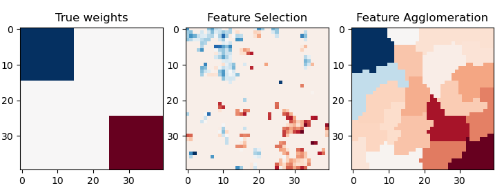
Feature agglomeration vs. univariate selection

This example compares 2 dimensionality reduction strategies:

• univariate feature selection with Anova

• feature agglomeration with Ward hierarchical clustering

Both methods are compared in a regression problem using a BayesianRidge as supervised estimator.

# Author: Alexandre Gramfort <alexandre.gramfort@inria.fr>
# License: BSD 3 clause

import shutil
import tempfile

import matplotlib.pyplot as plt
import numpy as np
from joblib import Memory
from scipy import linalg, ndimage

from sklearn import feature_selection
from sklearn.cluster import FeatureAgglomeration
from sklearn.feature_extraction.image import grid_to_graph
from sklearn.linear_model import BayesianRidge
from sklearn.model_selection import GridSearchCV, KFold
from sklearn.pipeline import Pipeline

Set parameters

n_samples = 200
size = 40  # image size
roi_size = 15
snr = 5.0
np.random.seed(0)

Generate data

coef = np.zeros((size, size))
coef[0:roi_size, 0:roi_size] = -1.0
coef[-roi_size:, -roi_size:] = 1.0

X = np.random.randn(n_samples, size**2)
for x in X:  # smooth data
    x[:] = ndimage.gaussian_filter(x.reshape(size, size), sigma=1.0).ravel()
X -= X.mean(axis=0)
X /= X.std(axis=0)

y = np.dot(X, coef.ravel())

add noise

noise = np.random.randn(y.shape[0])
noise_coef = (linalg.norm(y, 2) / np.exp(snr / 20.0)) / linalg.norm(noise, 2)
y += noise_coef * noise

Compute the coefs of a Bayesian Ridge with GridSearch

cv = KFold(2)  # cross-validation generator for model selection
ridge = BayesianRidge()
cachedir = tempfile.mkdtemp()
mem = Memory(location=cachedir, verbose=1)

Ward agglomeration followed by BayesianRidge

connectivity = grid_to_graph(n_x=size, n_y=size)
ward = FeatureAgglomeration(n_clusters=10, connectivity=connectivity, memory=mem)
clf = Pipeline([("ward", ward), ("ridge", ridge)])
# Select the optimal number of parcels with grid search
clf = GridSearchCV(clf, {"ward__n_clusters": [10, 20, 30]}, n_jobs=1, cv=cv)
clf.fit(X, y)  # set the best parameters
coef_ = clf.best_estimator_.steps[-1][1].coef_
coef_ = clf.best_estimator_.steps[0][1].inverse_transform(coef_)
coef_agglomeration_ = coef_.reshape(size, size)

________________________________________________________________________________
[Memory] Calling sklearn.cluster._agglomerative.ward_tree...
ward_tree(array([[-0.451933, ..., -0.675318],
       ...,
       [ 0.275706, ..., -1.085711]]), connectivity=<1600x1600 sparse matrix of type '<class 'numpy.int64'>'
        with 7840 stored elements in COOrdinate format>, n_clusters=None, return_distance=False)
________________________________________________________ward_tree - 0.0s, 0.0min
________________________________________________________________________________
[Memory] Calling sklearn.cluster._agglomerative.ward_tree...
ward_tree(array([[ 0.905206, ...,  0.161245],
       ...,
       [-0.849835, ..., -1.091621]]), connectivity=<1600x1600 sparse matrix of type '<class 'numpy.int64'>'
        with 7840 stored elements in COOrdinate format>, n_clusters=None, return_distance=False)
________________________________________________________ward_tree - 0.0s, 0.0min
________________________________________________________________________________
[Memory] Calling sklearn.cluster._agglomerative.ward_tree...
ward_tree(array([[ 0.905206, ..., -0.675318],
       ...,
       [-0.849835, ..., -1.085711]]), connectivity=<1600x1600 sparse matrix of type '<class 'numpy.int64'>'
        with 7840 stored elements in COOrdinate format>, n_clusters=None, return_distance=False)
________________________________________________________ward_tree - 0.0s, 0.0min

Anova univariate feature selection followed by BayesianRidge

f_regression = mem.cache(feature_selection.f_regression)  # caching function
anova = feature_selection.SelectPercentile(f_regression)
clf = Pipeline([("anova", anova), ("ridge", ridge)])
# Select the optimal percentage of features with grid search
clf = GridSearchCV(clf, {"anova__percentile": [5, 10, 20]}, cv=cv)
clf.fit(X, y)  # set the best parameters
coef_ = clf.best_estimator_.steps[-1][1].coef_
coef_ = clf.best_estimator_.steps[0][1].inverse_transform(coef_.reshape(1, -1))
coef_selection_ = coef_.reshape(size, size)

________________________________________________________________________________
[Memory] Calling sklearn.feature_selection._univariate_selection.f_regression...
f_regression(array([[-0.451933, ...,  0.275706],
       ...,
       [-0.675318, ..., -1.085711]]),
array([ 25.267703, ..., -25.026711]))
_____________________________________________________f_regression - 0.0s, 0.0min
________________________________________________________________________________
[Memory] Calling sklearn.feature_selection._univariate_selection.f_regression...
f_regression(array([[ 0.905206, ..., -0.849835],
       ...,
       [ 0.161245, ..., -1.091621]]),
array([ -27.447268, ..., -112.638768]))
_____________________________________________________f_regression - 0.0s, 0.0min
________________________________________________________________________________
[Memory] Calling sklearn.feature_selection._univariate_selection.f_regression...
f_regression(array([[ 0.905206, ..., -0.849835],
       ...,
       [-0.675318, ..., -1.085711]]),
array([-27.447268, ..., -25.026711]))
_____________________________________________________f_regression - 0.0s, 0.0min

Inverse the transformation to plot the results on an image

plt.close("all")
plt.figure(figsize=(7.3, 2.7))
plt.subplot(1, 3, 1)
plt.imshow(coef, interpolation="nearest", cmap=plt.cm.RdBu_r)
plt.title("True weights")
plt.subplot(1, 3, 2)
plt.imshow(coef_selection_, interpolation="nearest", cmap=plt.cm.RdBu_r)
plt.title("Feature Selection")
plt.subplot(1, 3, 3)
plt.imshow(coef_agglomeration_, interpolation="nearest", cmap=plt.cm.RdBu_r)
plt.title("Feature Agglomeration")
plt.subplots_adjust(0.04, 0.0, 0.98, 0.94, 0.16, 0.26)
plt.show()

Attempt to remove the temporary cachedir, but don’t worry if it fails

shutil.rmtree(cachedir, ignore_errors=True)

Related examples

A demo of structured Ward hierarchical clustering on an image of coins

A demo of structured Ward hierarchical clustering on an image of coins

HuberRegressor vs Ridge on dataset with strong outliers

HuberRegressor vs Ridge on dataset with strong outliers

Train error vs Test error

Train error vs Test error

Univariate Feature Selection

Univariate Feature Selection

Orthogonal Matching Pursuit

Orthogonal Matching Pursuit