Note
Go to the end to download the full example code or to run this example in your browser via JupyterLite or Binder.
Ordinary Least Squares and Ridge Regression#
Ordinary Least Squares: We illustrate how to use the ordinary least squares (OLS) model,
LinearRegression, on a single feature of the diabetes dataset. We train on a subset of the data, evaluate on a test set, and visualize the predictions.Ordinary Least Squares and Ridge Regression Variance: We then show how OLS can have high variance when the data is sparse or noisy, by fitting on a very small synthetic sample repeatedly. Ridge regression,
Ridge, reduces this variance by penalizing (shrinking) the coefficients, leading to more stable predictions.
# Authors: The scikit-learn developers
# SPDX-License-Identifier: BSD-3-Clause
Data Loading and Preparation#
Load the diabetes dataset. For simplicity, we only keep a single feature in the data. Then, we split the data and target into training and test sets.
from sklearn.datasets import load_diabetes
from sklearn.model_selection import train_test_split

X, y = load_diabetes(return_X_y=True)
X = X[:, [2]]  # Use only one feature
X_train, X_test, y_train, y_test = train_test_split(X, y, test_size=20, shuffle=False)
Linear regression model#
We create a linear regression model and fit it on the training data. Note that by
default, an intercept is added to the model. We can control this behavior by setting
the fit_intercept parameter.
from sklearn.linear_model import LinearRegression

regressor = LinearRegression().fit(X_train, y_train)
Model evaluation#
We evaluate the model’s performance on the test set using the mean squared error and the coefficient of determination.
from sklearn.metrics import mean_squared_error, r2_score

y_pred = regressor.predict(X_test)

print(f"Mean squared error: {mean_squared_error(y_test, y_pred):.2f}")
print(f"Coefficient of determination: {r2_score(y_test, y_pred):.2f}")
Mean squared error: 2548.07
Coefficient of determination: 0.47
Plotting the results#
Finally, we visualize the results on the train and test data.
import matplotlib.pyplot as plt

fig, ax = plt.subplots(ncols=2, figsize=(10, 5), sharex=True, sharey=True)

ax[0].scatter(X_train, y_train, label="Train data points")
ax[0].plot(
    X_train,
    regressor.predict(X_train),
    linewidth=3,
    color="tab:orange",
    label="Model predictions",
)
ax[0].set(xlabel="Feature", ylabel="Target", title="Train set")
ax[0].legend()

ax[1].scatter(X_test, y_test, label="Test data points")
ax[1].plot(X_test, y_pred, linewidth=3, color="tab:orange", label="Model predictions")
ax[1].set(xlabel="Feature", ylabel="Target", title="Test set")
ax[1].legend()

fig.suptitle("Linear Regression")

plt.show()
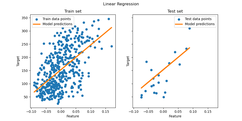
OLS on this single-feature subset learns a linear function that minimizes the mean squared error on the training data. We can see how well (or poorly) it generalizes by looking at the R^2 score and mean squared error on the test set. In higher dimensions, pure OLS often overfits, especially if the data is noisy. Regularization techniques (like Ridge or Lasso) can help reduce that.
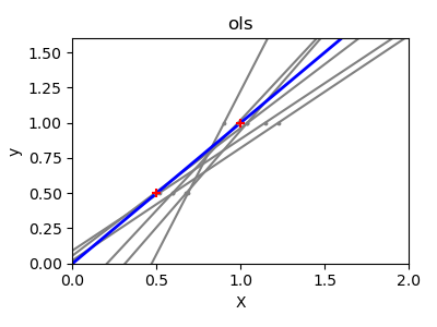
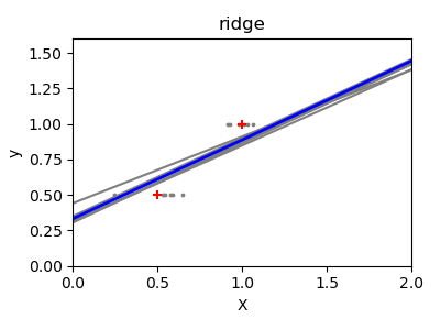
Ordinary Least Squares and Ridge Regression Variance#
Next, we illustrate the problem of high variance more clearly by using a tiny synthetic dataset. We sample only two data points, then repeatedly add small Gaussian noise to them and refit both OLS and Ridge. We plot each new line to see how much OLS can jump around, whereas Ridge remains more stable thanks to its penalty term.
import matplotlib.pyplot as plt
import numpy as np

from sklearn import linear_model

X_train = np.c_[0.5, 1].T
y_train = [0.5, 1]
X_test = np.c_[0, 2].T

np.random.seed(0)

classifiers = dict(
    ols=linear_model.LinearRegression(), ridge=linear_model.Ridge(alpha=0.1)
)

for name, clf in classifiers.items():
    fig, ax = plt.subplots(figsize=(4, 3))

    for _ in range(6):
        this_X = 0.1 * np.random.normal(size=(2, 1)) + X_train
        clf.fit(this_X, y_train)

        ax.plot(X_test, clf.predict(X_test), color="gray")
        ax.scatter(this_X, y_train, s=3, c="gray", marker="o", zorder=10)

    clf.fit(X_train, y_train)
    ax.plot(X_test, clf.predict(X_test), linewidth=2, color="blue")
    ax.scatter(X_train, y_train, s=30, c="red", marker="+", zorder=10)

    ax.set_title(name)
    ax.set_xlim(0, 2)
    ax.set_ylim((0, 1.6))
    ax.set_xlabel("X")
    ax.set_ylabel("y")

    fig.tight_layout()

plt.show()
Conclusion#
In the first example, we applied OLS to a real dataset, showing how a plain linear model can fit the data by minimizing the squared error on the training set.
In the second example, OLS lines varied drastically each time noise was added, reflecting its high variance when data is sparse or noisy. By contrast, Ridge regression introduces a regularization term that shrinks the coefficients, stabilizing predictions.
Techniques like Ridge or
Lasso (which applies an L1 penalty) are both
common ways to improve generalization and reduce overfitting. A well-tuned
Ridge or Lasso often outperforms pure OLS when features are correlated, data
is noisy, or sample size is small.
Total running time of the script: (0 minutes 0.382 seconds)
Related examples
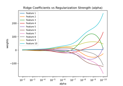
Plot Ridge coefficients as a function of the regularization
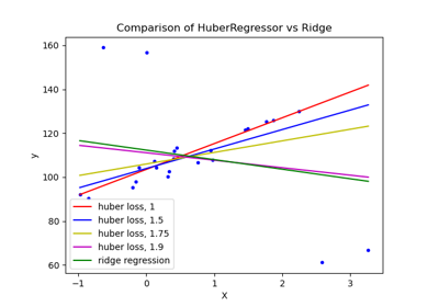
HuberRegressor vs Ridge on dataset with strong outliers
Comparison of kernel ridge and Gaussian process regression
