Combine predictors using stacking

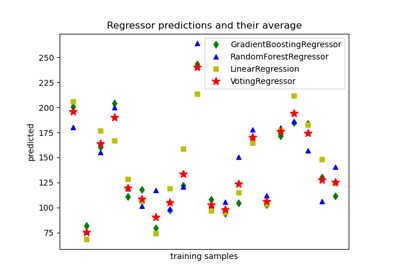
Stacking is an ensemble method. In this strategy, the out-of-fold predictions from several base estimators are used to train a meta-model that combines their outputs at inference time. Unlike VotingRegressor, which averages predictions with fixed (optionally user-specified) weights, StackingRegressor learns the combination through its final_estimator.

In this example, we illustrate the use case in which different regressors are stacked together and a final regularized linear regressor is used to output the prediction. We compare the performance of each individual regressor with the stacking strategy. Here, stacking slightly improves the overall performance.

# Authors: The scikit-learn developers
# SPDX-License-Identifier: BSD-3-Clause

Generate data

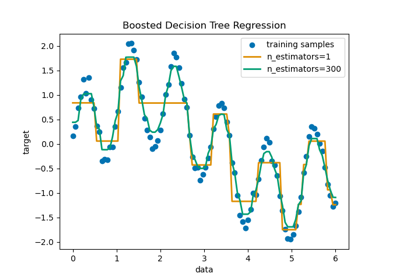
We use synthetic data generated from a sinusoid plus a linear trend with heteroscedastic Gaussian noise. A sudden drop is introduced, as it cannot be described by a linear model, but a tree-based model can naturally deal with it.

import numpy as np
import pandas as pd

rng = np.random.RandomState(42)
X = rng.uniform(-3, 3, size=500)
trend = 2.4 * X
seasonal = 3.1 * np.sin(3.2 * X)
drop = 10.0 * (X > 2).astype(float)
sigma = 0.75 + 0.75 * X**2
y = trend + seasonal - drop + rng.normal(loc=0.0, scale=np.sqrt(sigma))

df = pd.DataFrame({"X": X, "y": y})
_ = df.plot.scatter(x="X", y="y")

Stack of predictors on a single data set

It is sometimes not evident which model is more suited for a given task, as different model families can achieve similar performance while exhibiting different strengths and weaknesses. Stacking combines their outputs to exploit these complementary behaviors and can correct systematic errors that no single model can fix on its own. With appropriate regularization in the final_estimator, the StackingRegressor often matches the strongest base model, and can outperform it when base learners’ errors are only partially correlated, allowing the combination to reduce individual bias/variance.

Here, we combine 3 learners (linear and non-linear) and use the default RidgeCV regressor to combine their outputs together.

Note

Although some base learners include preprocessing (such as the StandardScaler), the final_estimator does not need additional preprocessing when using the default passthrough=False, as it receives only the base learners’ predictions. If passthrough=True, final_estimator should be a pipeline with proper preprocessing.

from sklearn.ensemble import HistGradientBoostingRegressor, StackingRegressor
from sklearn.linear_model import RidgeCV
from sklearn.pipeline import make_pipeline
from sklearn.preprocessing import PolynomialFeatures, SplineTransformer, StandardScaler

linear_ridge = make_pipeline(StandardScaler(), RidgeCV())

spline_ridge = make_pipeline(
    SplineTransformer(n_knots=6, degree=3),
    PolynomialFeatures(interaction_only=True),
    RidgeCV(),
)

hgbt = HistGradientBoostingRegressor(random_state=0)

estimators = [
    ("Linear Ridge", linear_ridge),
    ("Spline Ridge", spline_ridge),
    ("HGBT", hgbt),
]

stacking_regressor = StackingRegressor(estimators=estimators, final_estimator=RidgeCV())
stacking_regressor

StackingRegressor(estimators=[('Linear Ridge',
                               Pipeline(steps=[('standardscaler',
                                                StandardScaler()),
                                               ('ridgecv', RidgeCV())])),
                              ('Spline Ridge',
                               Pipeline(steps=[('splinetransformer',
                                                SplineTransformer(n_knots=6)),
                                               ('polynomialfeatures',
                                                PolynomialFeatures(interaction_only=True)),
                                               ('ridgecv', RidgeCV())])),
                              ('HGBT',
                               HistGradientBoostingRegressor(random_state=0))],
                  final_estimator=RidgeCV())

In a Jupyter environment, please rerun this cell to show the HTML representation or trust the notebook.
On GitHub, the HTML representation is unable to render, please try loading this page with nbviewer.org.

Measure and plot the results

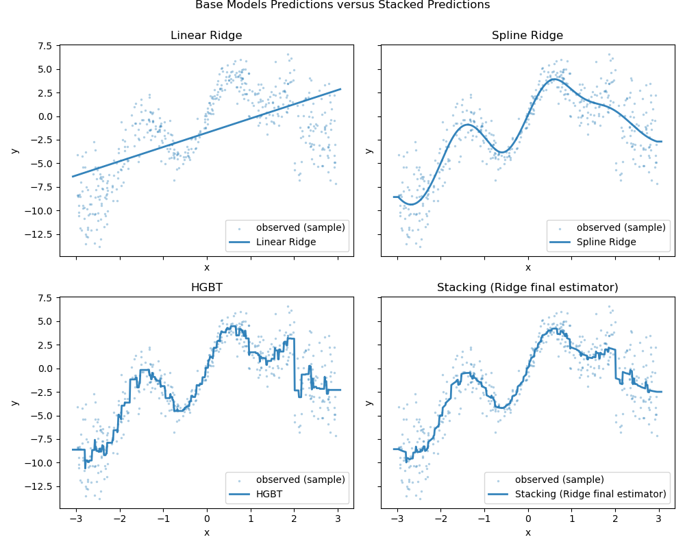
We can directly plot the predictions. Indeed, the sudden drop is correctly described by the HistGradientBoostingRegressor model (HGBT), but the spline model is smoother and less overfitting. The stacked regressor then turns to be a smoother version of the HGBT.

import matplotlib.pyplot as plt

X = X.reshape(-1, 1)
linear_ridge.fit(X, y)
spline_ridge.fit(X, y)
hgbt.fit(X, y)
stacking_regressor.fit(X, y)

x_plot = np.linspace(X.min() - 0.1, X.max() + 0.1, 500).reshape(-1, 1)
preds = {
    "Linear Ridge": linear_ridge.predict(x_plot),
    "Spline Ridge": spline_ridge.predict(x_plot),
    "HGBT": hgbt.predict(x_plot),
    "Stacking (Ridge final estimator)": stacking_regressor.predict(x_plot),
}

fig, axes = plt.subplots(2, 2, figsize=(10, 8), sharex=True, sharey=True)
axes = axes.ravel()
for ax, (name, y_pred) in zip(axes, preds.items()):
    ax.scatter(
        X[:, 0],
        y,
        s=6,
        alpha=0.35,
        linewidths=0,
        label="observed (sample)",
    )

    ax.plot(x_plot.ravel(), y_pred, linewidth=2, alpha=0.9, label=name)
    ax.set_title(name)
    ax.set_xlabel("x")
    ax.set_ylabel("y")
    ax.legend(loc="lower right")

plt.suptitle("Base Models Predictions versus Stacked Predictions", y=1)
plt.tight_layout()
plt.show()

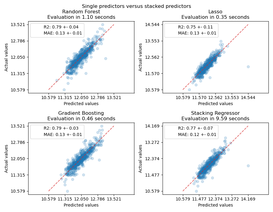
We can plot the prediction errors as well and evaluate the performance of the individual predictors and the stack of the regressors.

import time

from sklearn.metrics import PredictionErrorDisplay
from sklearn.model_selection import cross_val_predict, cross_validate

fig, axs = plt.subplots(2, 2, figsize=(9, 7))
axs = np.ravel(axs)

for ax, (name, est) in zip(
    axs, estimators + [("Stacking Regressor", stacking_regressor)]
):
    scorers = {r"$R^2$": "r2", "MAE": "neg_mean_absolute_error"}

    start_time = time.time()
    scores = cross_validate(est, X, y, scoring=list(scorers.values()), n_jobs=-1)
    elapsed_time = time.time() - start_time

    y_pred = cross_val_predict(est, X, y, n_jobs=-1)
    scores = {
        key: (
            f"{np.abs(np.mean(scores[f'test_{value}'])):.2f}"
            r" $\pm$ "
            f"{np.std(scores[f'test_{value}']):.2f}"
        )
        for key, value in scorers.items()
    }

    display = PredictionErrorDisplay.from_predictions(
        y_true=y,
        y_pred=y_pred,
        kind="actual_vs_predicted",
        ax=ax,
        scatter_kwargs={"alpha": 0.2, "color": "tab:blue"},
        line_kwargs={"color": "tab:red"},
    )
    ax.set_title(f"{name}\nEvaluation in {elapsed_time:.2f} seconds")

    for name, score in scores.items():
        ax.plot([], [], " ", label=f"{name}: {score}")
    ax.legend(loc="upper left")

plt.suptitle("Prediction Errors of Base versus Stacked Predictors", y=1)
plt.tight_layout()
plt.subplots_adjust(top=0.9)
plt.show()

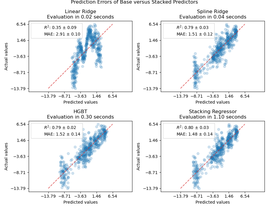
Even if the scores overlap considerably after cross-validation, the predictions from the stacked regressor are slightly better.

Once fitted, we can inspect the coefficients (or meta-weights) of the trained final_estimator_ (as long as it is a linear model). They reveal how much the individual estimators contribute to the the stacked regressor:

stacking_regressor.fit(X, y)
stacking_regressor.final_estimator_.coef_

array([-0.00470849,  0.44997974,  0.54915302])

We see that in this case, the HGBT model dominates, with the spline ridge also contributing meaningfully. The plain linear model does not add useful signal once those two are included; with RidgeCV as the final_estimator, it is not dropped, but receives a small negative weight to correct its residual bias.

If we use LassoCV as the final_estimator, that small, unhelpful contribution is set exactly to zero, yielding a simpler blend of the spline ridge and HGBT models.

from sklearn.linear_model import LassoCV

stacking_regressor = StackingRegressor(estimators=estimators, final_estimator=LassoCV())
stacking_regressor.fit(X, y)
stacking_regressor.final_estimator_.coef_

array([0.        , 0.41537408, 0.56077966])

How to mimic SuperLearner with scikit-learn

The SuperLearner [Polley2010] is a stacking strategy implemented as an R package, but not available off-the-shelf in Python. It is closely related to the StackingRegressor, as both train the meta-model on out-of-fold predictions from the base estimators.

The key difference is that SuperLearner estimates a convex set of meta-weights (non-negative and summing to 1) and omits an intercept; by contrast, StackingRegressor uses an unconstrained meta-learner with an intercept by default (and can optionally include raw features via passthrough).

Without an intercept, the meta-weights are directly interpretable as fractional contributions to the final prediction.

from sklearn.linear_model import LinearRegression

linear_reg = LinearRegression(fit_intercept=False, positive=True)
super_learner_like = StackingRegressor(
    estimators=estimators, final_estimator=linear_reg
)
super_learner_like.fit(X, y)
super_learner_like.final_estimator_.coef_

array([0.        , 0.44466993, 0.55303985])

The sum of meta-weights in the stacked regressor is close to 1.0, but not exactly one:

super_learner_like.final_estimator_.coef_.sum()

np.float64(0.9977097805095475)

Beyond interpretability, the normalization to 1.0 constraint in the SuperLearner presents the following advantages:

• Consensus-preserving: if all base models output the same value at a point, the ensemble returns that same value (no artificial amplification or attenuation).

• Translation-equivariant: adding a constant to every base prediction shifts the ensemble by the same constant.

• Removes one degree of freedom: avoiding redundancy with a constant term and modestly stabilizing weights under collinearity.

The cleanest way to enforce the coefficient normalization with scikit-learn is by defining a custom estimator, but doing so is beyond the scope of this tutorial.

Conclusions

The stacked regressor combines the strengths of the different regressors. However, notice that training the stacked regressor is much more computationally expensive than selecting the best performing model.

References

[Polley2010]

Polley, E. C. and van der Laan, M. J., Super Learner In Prediction, 2010.

Related examples

Plot individual and voting regression predictions

Plot individual and voting regression predictions

Features in Histogram Gradient Boosting Trees

Features in Histogram Gradient Boosting Trees

Decision Tree Regression with AdaBoost

Decision Tree Regression with AdaBoost

Polynomial and Spline interpolation

Polynomial and Spline interpolation