Note

Go to the end to download the full example code or to run this example in your browser via JupyterLite or Binder

Release Highlights for scikit-learn 1.3¶

We are pleased to announce the release of scikit-learn 1.3! Many bug fixes and improvements were added, as well as some new key features. We detail below a few of the major features of this release. For an exhaustive list of all the changes, please refer to the release notes.

To install the latest version (with pip):

pip install --upgrade scikit-learn

or with conda:

conda install -c conda-forge scikit-learn

Metadata Routing¶

We are in the process of introducing a new way to route metadata such as sample_weight throughout the codebase, which would affect how meta-estimators such as pipeline.Pipeline and model_selection.GridSearchCV route metadata. While the infrastructure for this feature is already included in this release, the work is ongoing and not all meta-estimators support this new feature. You can read more about this feature in the Metadata Routing User Guide. Note that this feature is still under development and not implemented for most meta-estimators.

Third party developers can already start incorporating this into their meta-estimators. For more details, see metadata routing developer guide.

HDBSCAN: hierarchical density-based clustering¶

Originally hosted in the scikit-learn-contrib repository, cluster.HDBSCAN has been adpoted into scikit-learn. It’s missing a few features from the original implementation which will be added in future releases. By performing a modified version of cluster.DBSCAN over multiple epsilon values simultaneously, cluster.HDBSCAN finds clusters of varying densities making it more robust to parameter selection than cluster.DBSCAN. More details in the User Guide.

import numpy as np
from sklearn.cluster import HDBSCAN
from sklearn.datasets import load_digits
from sklearn.metrics import v_measure_score

X, true_labels = load_digits(return_X_y=True)
print(f"number of digits: {len(np.unique(true_labels))}")

hdbscan = HDBSCAN(min_cluster_size=15).fit(X)
non_noisy_labels = hdbscan.labels_[hdbscan.labels_ != -1]
print(f"number of clusters found: {len(np.unique(non_noisy_labels))}")

print(v_measure_score(true_labels[hdbscan.labels_ != -1], non_noisy_labels))

number of digits: 10
number of clusters found: 11
0.9694149248180188

TargetEncoder: a new category encoding strategy¶

Well suited for categorical features with high cardinality, preprocessing.TargetEncoder encodes the categories based on a shrunk estimate of the average target values for observations belonging to that category. More details in the User Guide.

import numpy as np
from sklearn.preprocessing import TargetEncoder

X = np.array([["cat"] * 30 + ["dog"] * 20 + ["snake"] * 38], dtype=object).T
y = [90.3] * 30 + [20.4] * 20 + [21.2] * 38

enc = TargetEncoder(random_state=0)
X_trans = enc.fit_transform(X, y)

enc.encodings_

[array([90.3, 20.4, 21.2])]

Missing values support in decision trees¶

The classes tree.DecisionTreeClassifier and tree.DecisionTreeRegressor now support missing values. For each potential threshold on the non-missing data, the splitter will evaluate the split with all the missing values going to the left node or the right node. See more details in the User Guide or see Features in Histogram Gradient Boosting Trees for a usecase example of this feature in HistGradientBoostingRegressor.

import numpy as np
from sklearn.tree import DecisionTreeClassifier

X = np.array([0, 1, 6, np.nan]).reshape(-1, 1)
y = [0, 0, 1, 1]

tree = DecisionTreeClassifier(random_state=0).fit(X, y)
tree.predict(X)

array([0, 0, 1, 1])

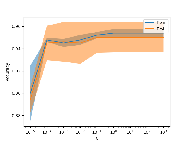
New display `model_selection.ValidationCurveDisplay`¶

model_selection.ValidationCurveDisplay is now available to plot results from model_selection.validation_curve.

from sklearn.datasets import make_classification
from sklearn.linear_model import LogisticRegression
from sklearn.model_selection import ValidationCurveDisplay

X, y = make_classification(1000, 10, random_state=0)

_ = ValidationCurveDisplay.from_estimator(
    LogisticRegression(),
    X,
    y,
    param_name="C",
    param_range=np.geomspace(1e-5, 1e3, num=9),
    score_type="both",
    score_name="Accuracy",
)

Gamma loss for gradient boosting¶

The class ensemble.HistGradientBoostingRegressor supports the Gamma deviance loss function via loss="gamma". This loss function is useful for modeling strictly positive targets with a right-skewed distribution.

import numpy as np
from sklearn.model_selection import cross_val_score
from sklearn.datasets import make_low_rank_matrix
from sklearn.ensemble import HistGradientBoostingRegressor

n_samples, n_features = 500, 10
rng = np.random.RandomState(0)
X = make_low_rank_matrix(n_samples, n_features, random_state=rng)
coef = rng.uniform(low=-10, high=20, size=n_features)
y = rng.gamma(shape=2, scale=np.exp(X @ coef) / 2)
gbdt = HistGradientBoostingRegressor(loss="gamma")
cross_val_score(gbdt, X, y).mean()

0.46858513287221654

Grouping infrequent categories in `preprocessing.OrdinalEncoder`¶

Similarly to preprocessing.OneHotEncoder, the class preprocessing.OrdinalEncoder now supports aggregating infrequent categories into a single output for each feature. The parameters to enable the gathering of infrequent categories are min_frequency and max_categories. See the User Guide for more details.

from sklearn.preprocessing import OrdinalEncoder
import numpy as np

X = np.array(
    [["dog"] * 5 + ["cat"] * 20 + ["rabbit"] * 10 + ["snake"] * 3], dtype=object
).T
enc = OrdinalEncoder(min_frequency=6).fit(X)
enc.infrequent_categories_