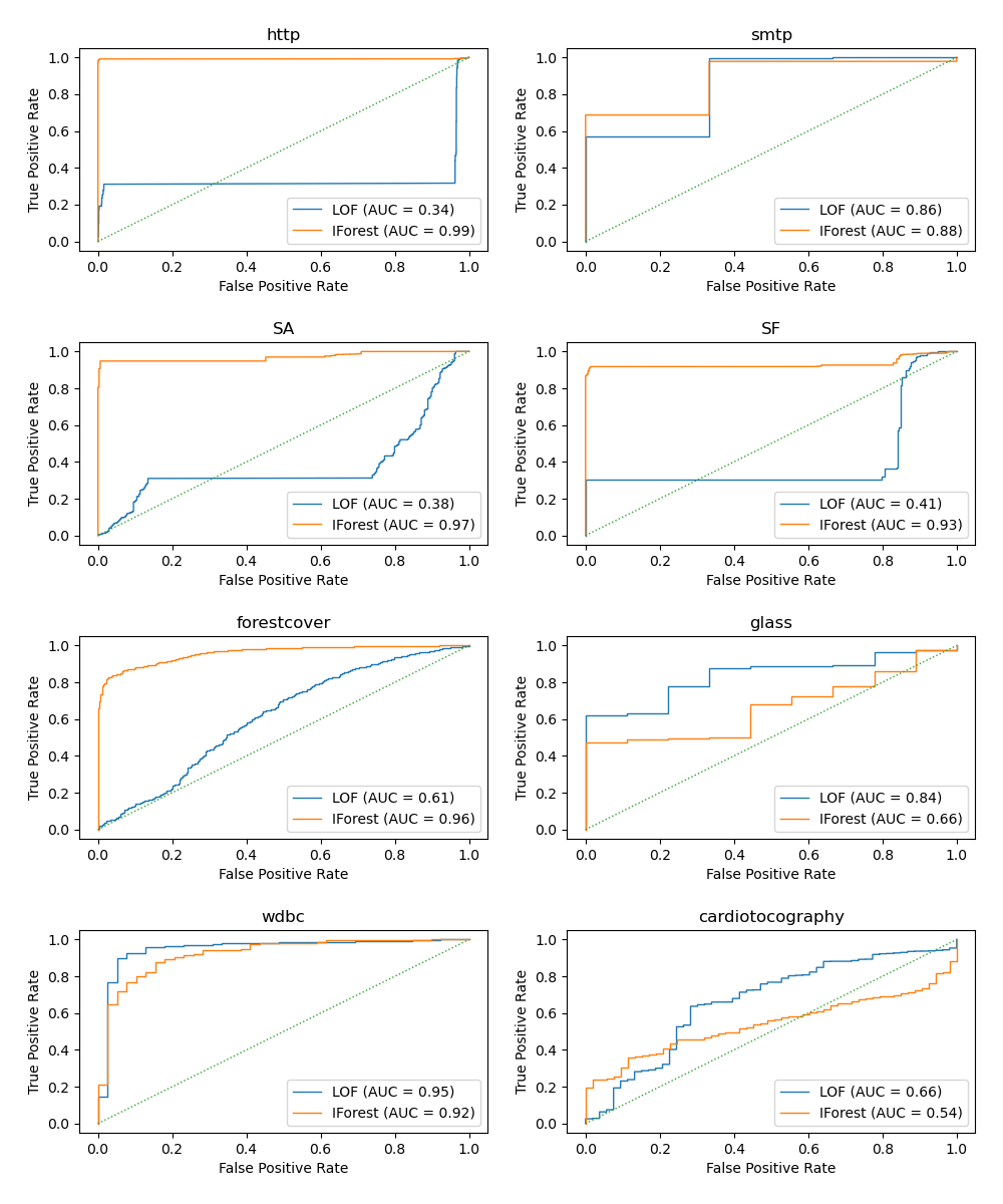
Evaluation of outlier detection estimators

This example benchmarks outlier detection algorithms, Local Outlier Factor (LOF) and Isolation Forest (IForest), using ROC curves on classical anomaly detection datasets. The algorithm performance is assessed in an outlier detection context:

1. The algorithms are trained on the whole dataset which is assumed to contain outliers.

2. The ROC curve from RocCurveDisplay is computed on the same dataset using the knowledge of the labels.

# Author: Pharuj Rajborirug <pharuj.ra@kmitl.ac.th>
# License: BSD 3 clause

print(__doc__)

Define a data preprocessing function

The example uses real-world datasets available in sklearn.datasets and the sample size of some datasets is reduced to speed up computation. After the data preprocessing, the datasets’ targets will have two classes, 0 representing inliers and 1 representing outliers. The preprocess_dataset function returns data and target.

import numpy as np
from sklearn.datasets import fetch_kddcup99, fetch_covtype, fetch_openml
from sklearn.preprocessing import LabelBinarizer
import pandas as pd

rng = np.random.RandomState(42)


def preprocess_dataset(dataset_name):

    # loading and vectorization
    print(f"Loading {dataset_name} data")
    if dataset_name in ["http", "smtp", "SA", "SF"]:
        dataset = fetch_kddcup99(subset=dataset_name, percent10=True, random_state=rng)
        X = dataset.data
        y = dataset.target
        lb = LabelBinarizer()

        if dataset_name == "SF":
            idx = rng.choice(X.shape[0], int(X.shape[0] * 0.1), replace=False)
            X = X[idx]  # reduce the sample size
            y = y[idx]
            x1 = lb.fit_transform(X[:, 1].astype(str))
            X = np.c_[X[:, :1], x1, X[:, 2:]]
        elif dataset_name == "SA":
            idx = rng.choice(X.shape[0], int(X.shape[0] * 0.1), replace=False)
            X = X[idx]  # reduce the sample size
            y = y[idx]
            x1 = lb.fit_transform(X[:, 1].astype(str))
            x2 = lb.fit_transform(X[:, 2].astype(str))
            x3 = lb.fit_transform(X[:, 3].astype(str))
            X = np.c_[X[:, :1], x1, x2, x3, X[:, 4:]]
        y = (y != b"normal.").astype(int)
    if dataset_name == "forestcover":
        dataset = fetch_covtype()
        X = dataset.data
        y = dataset.target
        idx = rng.choice(X.shape[0], int(X.shape[0] * 0.1), replace=False)
        X = X[idx]  # reduce the sample size
        y = y[idx]

        # inliers are those with attribute 2
        # outliers are those with attribute 4
        s = (y == 2) + (y == 4)
        X = X[s, :]
        y = y[s]
        y = (y != 2).astype(int)
    if dataset_name in ["glass", "wdbc", "cardiotocography"]:
        dataset = fetch_openml(
            name=dataset_name, version=1, as_frame=False, parser="pandas"
        )
        X = dataset.data
        y = dataset.target

        if dataset_name == "glass":
            s = y == "tableware"
            y = s.astype(int)
        if dataset_name == "wdbc":
            s = y == "2"
            y = s.astype(int)
            X_mal, y_mal = X[s], y[s]
            X_ben, y_ben = X[~s], y[~s]

            # downsampled to 39 points (9.8% outliers)
            idx = rng.choice(y_mal.shape[0], 39, replace=False)
            X_mal2 = X_mal[idx]
            y_mal2 = y_mal[idx]
            X = np.concatenate((X_ben, X_mal2), axis=0)
            y = np.concatenate((y_ben, y_mal2), axis=0)
        if dataset_name == "cardiotocography":
            s = y == "3"
            y = s.astype(int)
    # 0 represents inliers, and 1 represents outliers
    y = pd.Series(y, dtype="category")
    return (X, y)

Define an outlier prediction function

There is no particular reason to choose algorithms LocalOutlierFactor and IsolationForest. The goal is to show that different algorithm performs well on different datasets. The following compute_prediction function returns average outlier score of X.

from sklearn.neighbors import LocalOutlierFactor
from sklearn.ensemble import IsolationForest


def compute_prediction(X, model_name):

    print(f"Computing {model_name} prediction...")
    if model_name == "LOF":
        clf = LocalOutlierFactor(n_neighbors=20, contamination="auto")
        clf.fit(X)
        y_pred = clf.negative_outlier_factor_
    if model_name == "IForest":
        clf = IsolationForest(random_state=rng, contamination="auto")
        y_pred = clf.fit(X).decision_function(X)
    return y_pred

Plot and interpret results

The algorithm performance relates to how good the true positive rate (TPR) is at low value of the false positive rate (FPR). The best algorithms have the curve on the top-left of the plot and the area under curve (AUC) close to 1. The diagonal dashed line represents a random classification of outliers and inliers.

import math
import matplotlib.pyplot as plt
from sklearn.metrics import RocCurveDisplay

datasets_name = [
    "http",
    "smtp",
    "SA",
    "SF",
    "forestcover",
    "glass",
    "wdbc",
    "cardiotocography",
]

models_name = [
    "LOF",
    "IForest",
]

# plotting parameters
cols = 2
linewidth = 1
pos_label = 0  # mean 0 belongs to positive class
rows = math.ceil(len(datasets_name) / cols)

fig, axs = plt.subplots(rows, cols, figsize=(10, rows * 3))

for i, dataset_name in enumerate(datasets_name):
    (X, y) = preprocess_dataset(dataset_name=dataset_name)

    for model_name in models_name:
        y_pred = compute_prediction(X, model_name=model_name)
        display = RocCurveDisplay.from_predictions(
            y,
            y_pred,
            pos_label=pos_label,
            name=model_name,
            linewidth=linewidth,
            ax=axs[i // cols, i % cols],
        )
    axs[i // cols, i % cols].plot([0, 1], [0, 1], linewidth=linewidth, linestyle=":")
    axs[i // cols, i % cols].set_title(dataset_name)
    axs[i // cols, i % cols].set_xlabel("False Positive Rate")
    axs[i // cols, i % cols].set_ylabel("True Positive Rate")
plt.tight_layout(pad=2.0)  # spacing between subplots
plt.show()

Loading http data
Computing LOF prediction...
Computing IForest prediction...
Loading smtp data
Computing LOF prediction...
Computing IForest prediction...
Loading SA data
Computing LOF prediction...
Computing IForest prediction...
Loading SF data
Computing LOF prediction...
Computing IForest prediction...
Loading forestcover data
Computing LOF prediction...
Computing IForest prediction...
Loading glass data
Computing LOF prediction...
Computing IForest prediction...
Loading wdbc data
Computing LOF prediction...
Computing IForest prediction...
Loading cardiotocography data
Computing LOF prediction...
Computing IForest prediction...