sklearn.inspection.DecisionBoundaryDisplay

class sklearn.inspection.DecisionBoundaryDisplay(*, xx0, xx1, response, xlabel=None, ylabel=None)

Decisions boundary visualization.

It is recommended to use from_estimator to create a DecisionBoundaryDisplay. All parameters are stored as attributes.

Read more in the User Guide.

New in version 1.1.

Parameters:

xx0ndarray of shape (grid_resolution, grid_resolution)

First output of meshgrid.

xx1ndarray of shape (grid_resolution, grid_resolution)

Second output of meshgrid.

responsendarray of shape (grid_resolution, grid_resolution)

Values of the response function.

xlabelstr, default=None

Default label to place on x axis.

ylabelstr, default=None

Default label to place on y axis.

Attributes:

surface_matplotlib QuadContourSet or QuadMesh

If plot_method is ‘contour’ or ‘contourf’, surface_ is a QuadContourSet. If plot_method is ‘pcolormesh’, surface_ is a QuadMesh.

ax_matplotlib Axes

Axes with confusion matrix.

figure_matplotlib Figure

Figure containing the confusion matrix.

See also

DecisionBoundaryDisplay.from_estimator

Plot decision boundary given an estimator.

Examples

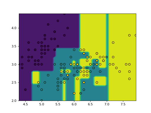
>>> import matplotlib.pyplot as plt
>>> import numpy as np
>>> from sklearn.datasets import load_iris
>>> from sklearn.inspection import DecisionBoundaryDisplay
>>> from sklearn.tree import DecisionTreeClassifier
>>> iris = load_iris()
>>> feature_1, feature_2 = np.meshgrid(
...     np.linspace(iris.data[:, 0].min(), iris.data[:, 0].max()),
...     np.linspace(iris.data[:, 1].min(), iris.data[:, 1].max())
... )
>>> grid = np.vstack([feature_1.ravel(), feature_2.ravel()]).T
>>> tree = DecisionTreeClassifier().fit(iris.data[:, :2], iris.target)
>>> y_pred = np.reshape(tree.predict(grid), feature_1.shape)
>>> display = DecisionBoundaryDisplay(
...     xx0=feature_1, xx1=feature_2, response=y_pred
... )
>>> display.plot()
<...>
>>> display.ax_.scatter(
...     iris.data[:, 0], iris.data[:, 1], c=iris.target, edgecolor="black"
... )
<...>
>>> plt.show()

Methods

from_estimator(estimator, X, *[, ...])	Plot decision boundary given an estimator.
plot([plot_method, ax, xlabel, ylabel])	Plot visualization.

classmethod from_estimator(estimator, X, *, grid_resolution=100, eps=1.0, plot_method='contourf', response_method='auto', xlabel=None, ylabel=None, ax=None, **kwargs)

Plot decision boundary given an estimator.

Read more in the User Guide.

Parameters:

estimatorobject

Trained estimator used to plot the decision boundary.

X{array-like, sparse matrix, dataframe} of shape (n_samples, 2)

Input data that should be only 2-dimensional.

grid_resolutionint, default=100

Number of grid points to use for plotting decision boundary. Higher values will make the plot look nicer but be slower to render.

epsfloat, default=1.0

Extends the minimum and maximum values of X for evaluating the response function.

plot_method{‘contourf’, ‘contour’, ‘pcolormesh’}, default=’contourf’

Plotting method to call when plotting the response. Please refer to the following matplotlib documentation for details: contourf, contour, pcolormesh.

response_method{‘auto’, ‘predict_proba’, ‘decision_function’, ‘predict’}, default=’auto’

Specifies whether to use predict_proba, decision_function, predict as the target response. If set to ‘auto’, the response method is tried in the following order: decision_function, predict_proba, predict. For multiclass problems, predict is selected when response_method="auto".

xlabelstr, default=None

The label used for the x-axis. If None, an attempt is made to extract a label from X if it is a dataframe, otherwise an empty string is used.

ylabelstr, default=None

The label used for the y-axis. If None, an attempt is made to extract a label from X if it is a dataframe, otherwise an empty string is used.

axMatplotlib axes, default=None

Axes object to plot on. If None, a new figure and axes is created.

**kwargsdict

Additional keyword arguments to be passed to the plot_method.

Returns:

displayDecisionBoundaryDisplay

Object that stores the result.

See also

DecisionBoundaryDisplay

Decision boundary visualization.

ConfusionMatrixDisplay.from_estimator

Plot the confusion matrix given an estimator, the data, and the label.

ConfusionMatrixDisplay.from_predictions

Plot the confusion matrix given the true and predicted labels.

Examples

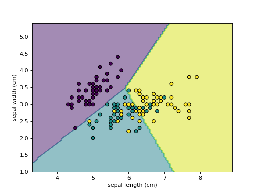
>>> import matplotlib.pyplot as plt
>>> from sklearn.datasets import load_iris
>>> from sklearn.linear_model import LogisticRegression
>>> from sklearn.inspection import DecisionBoundaryDisplay
>>> iris = load_iris()
>>> X = iris.data[:, :2]
>>> classifier = LogisticRegression().fit(X, iris.target)
>>> disp = DecisionBoundaryDisplay.from_estimator(
...     classifier, X, response_method="predict",
...     xlabel=iris.feature_names[0], ylabel=iris.feature_names[1],
...     alpha=0.5,
... )
>>> disp.ax_.scatter(X[:, 0], X[:, 1], c=iris.target, edgecolor="k")
<...>
>>> plt.show()

plot(plot_method='contourf', ax=None, xlabel=None, ylabel=None, **kwargs)

Plot visualization.

Parameters:

plot_method{‘contourf’, ‘contour’, ‘pcolormesh’}, default=’contourf’

Plotting method to call when plotting the response. Please refer to the following matplotlib documentation for details: contourf, contour, pcolormesh.

axMatplotlib axes, default=None

Axes object to plot on. If None, a new figure and axes is created.

xlabelstr, default=None

Overwrite the x-axis label.

ylabelstr, default=None

Overwrite the y-axis label.

**kwargsdict

Additional keyword arguments to be passed to the plot_method.

Returns:

display: DecisionBoundaryDisplay

Object that stores computed values.

Examples using sklearn.inspection.DecisionBoundaryDisplay

IsolationForest example

IsolationForest example