Note
Go to the end to download the full example code or to run this example in your browser via JupyterLite or Binder.
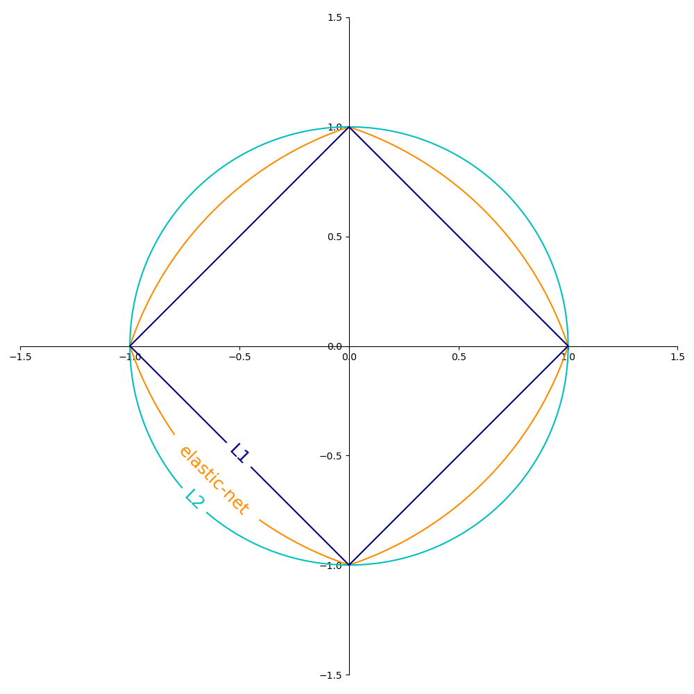
SGD: Penalties#
Contours of where the penalty is equal to 1 for the three penalties L1, L2 and elastic-net.
All of the above are supported by SGDClassifier
and SGDRegressor.
# Authors: The scikit-learn developers
# SPDX-License-Identifier: BSD-3-Clause

import matplotlib.pyplot as plt
import numpy as np

l1_color = "navy"
l2_color = "c"
elastic_net_color = "darkorange"

line = np.linspace(-1.5, 1.5, 1001)
xx, yy = np.meshgrid(line, line)

l2 = xx**2 + yy**2
l1 = np.abs(xx) + np.abs(yy)
rho = 0.5
elastic_net = rho * l1 + (1 - rho) * l2

plt.figure(figsize=(10, 10), dpi=100)
ax = plt.gca()

elastic_net_contour = plt.contour(
    xx, yy, elastic_net, levels=[1], colors=elastic_net_color
)
l2_contour = plt.contour(xx, yy, l2, levels=[1], colors=l2_color)
l1_contour = plt.contour(xx, yy, l1, levels=[1], colors=l1_color)
ax.set_aspect("equal")
ax.spines["left"].set_position("center")
ax.spines["right"].set_color("none")
ax.spines["bottom"].set_position("center")
ax.spines["top"].set_color("none")

plt.clabel(
    elastic_net_contour,
    inline=1,
    fontsize=18,
    fmt={1.0: "elastic-net"},
    manual=[(-1, -1)],
)
plt.clabel(l2_contour, inline=1, fontsize=18, fmt={1.0: "L2"}, manual=[(-1, -1)])
plt.clabel(l1_contour, inline=1, fontsize=18, fmt={1.0: "L1"}, manual=[(-1, -1)])

plt.tight_layout()
plt.show()
Total running time of the script: (0 minutes 0.238 seconds)
Related examples
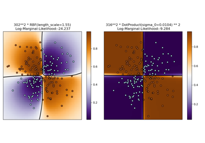
Illustration of Gaussian process classification (GPC) on the XOR dataset
Illustration of Gaussian process classification (GPC) on the XOR dataset
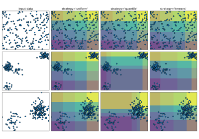
Demonstrating the different strategies of KBinsDiscretizer
Demonstrating the different strategies of KBinsDiscretizer
