Note

Go to the end to download the full example code or to run this example in your browser via JupyterLite or Binder.

Analysis of the convergence of penalized logistic regression models#

The purpose of this example is three-fold:

Demonstrate registering a ScoringMonitor on the logistic regression step of a pipeline nested inside GridSearchCV.
Show how to plot the metric values collected at each iteration of each fit of the logistic regression model during the grid search and analyze the convergence of the model for each hyperparameter combination.
Show how the monitoring of diverse scoring metrics can inform us about the quality of the model and the trade-off between refinement and calibration.

# Authors: The scikit-learn developers
# SPDX-License-Identifier: BSD-3-Clause

Setup#

Let’s first define the pipeline and the grid search. Here we register a ScoringMonitor callback on the logistic regression model to monitor the scores at each iteration of the L-BFGS solver.

We reuse the same scoring metrics for the grid search itself and use the D² log-loss as the primary metric to select the best hyperparameter combination.

import matplotlib.pyplot as plt
import numpy as np
import pandas as pd

from sklearn.callback import ProgressBar, ScoringMonitor
from sklearn.datasets import make_classification
from sklearn.linear_model import LogisticRegression
from sklearn.model_selection import GridSearchCV
from sklearn.pipeline import make_pipeline
from sklearn.preprocessing import StandardScaler

X, y = make_classification(
    n_samples=1000, n_features=100, n_classes=10, n_informative=30, random_state=42
)

scoring_metrics = ["d2_log_loss_score", "accuracy", "average_precision"]
scoring_monitor = ScoringMonitor(scoring=scoring_metrics)
model = make_pipeline(
    StandardScaler(),
    LogisticRegression(solver="lbfgs", max_iter=1000).set_callbacks(scoring_monitor),
)

param_grid = {
    "standardscaler__with_std": [True, False],
    "logisticregression__C": np.geomspace(0.01, 100, 3),
}

grid_search = GridSearchCV(
    model,
    param_grid,
    cv=5,
    scoring=scoring_metrics,
    n_jobs=2,
    error_score="raise",
    refit=scoring_metrics[0],
)

Let’s fit the grid search with the auto-propagating progress bar callback. Feel free to set max_propagation_depth=3 in the ProgressBar constructor to get a more detailed output by displaying the progress bars for the pipeline, the standard scaler and the logistic regression.

grid_search.set_callbacks(ProgressBar()).fit(X, y)

GridSearchCV - fit                                                 ━━━ 100% 0:0…
  GridSearchCV - search #0                                         ━━━ 100% 0:0…
    GridSearchCV - candidate-split-evaluation | Pipeline - fit #0  ━━━ 100% 0:0…
    GridSearchCV - candidate-split-evaluation | Pipeline - fit #1  ━━━ 100% 0:0…
    GridSearchCV - candidate-split-evaluation | Pipeline - fit #2  ━━━ 100% 0:0…
    GridSearchCV - candidate-split-evaluation | Pipeline - fit #3  ━━━ 100% 0:0…
    GridSearchCV - candidate-split-evaluation | Pipeline - fit #4  ━━━ 100% 0:0…
    GridSearchCV - candidate-split-evaluation | Pipeline - fit #5  ━━━ 100% 0:0…
    GridSearchCV - candidate-split-evaluation | Pipeline - fit #6  ━━━ 100% 0:0…
    GridSearchCV - candidate-split-evaluation | Pipeline - fit #7  ━━━ 100% 0:0…
    GridSearchCV - candidate-split-evaluation | Pipeline - fit #8  ━━━ 100% 0:0…
    GridSearchCV - candidate-split-evaluation | Pipeline - fit #9  ━━━ 100% 0:0…
    GridSearchCV - candidate-split-evaluation | Pipeline - fit #10 ━━━ 100% 0:0…
    GridSearchCV - candidate-split-evaluation | Pipeline - fit #11 ━━━ 100% 0:0…
    GridSearchCV - candidate-split-evaluation | Pipeline - fit #12 ━━━ 100% 0:0…
    GridSearchCV - candidate-split-evaluation | Pipeline - fit #13 ━━━ 100% 0:0…
    GridSearchCV - candidate-split-evaluation | Pipeline - fit #14 ━━━ 100% 0:0…
    GridSearchCV - candidate-split-evaluation | Pipeline - fit #15 ━━━ 100% 0:0…
    GridSearchCV - candidate-split-evaluation | Pipeline - fit #16 ━━━ 100% 0:0…
    GridSearchCV - candidate-split-evaluation | Pipeline - fit #17 ━━━ 100% 0:0…
    GridSearchCV - candidate-split-evaluation | Pipeline - fit #18 ━━━ 100% 0:0…
    GridSearchCV - candidate-split-evaluation | Pipeline - fit #19 ━━━ 100% 0:0…
    GridSearchCV - candidate-split-evaluation | Pipeline - fit #20 ━━━ 100% 0:0…
    GridSearchCV - candidate-split-evaluation | Pipeline - fit #21 ━━━ 100% 0:0…
    GridSearchCV - candidate-split-evaluation | Pipeline - fit #22 ━━━ 100% 0:0…
    GridSearchCV - candidate-split-evaluation | Pipeline - fit #23 ━━━ 100% 0:0…
    GridSearchCV - candidate-split-evaluation | Pipeline - fit #24 ━━━ 100% 0:0…
    GridSearchCV - candidate-split-evaluation | Pipeline - fit #25 ━━━ 100% 0:0…
    GridSearchCV - candidate-split-evaluation | Pipeline - fit #26 ━━━ 100% 0:0…
    GridSearchCV - candidate-split-evaluation | Pipeline - fit #27 ━━━ 100% 0:0…
    GridSearchCV - candidate-split-evaluation | Pipeline - fit #28 ━━━ 100% 0:0…
    GridSearchCV - candidate-split-evaluation | Pipeline - fit #29 ━━━ 100% 0:0…
  GridSearchCV - refit-with-best-params | Pipeline - fit #1        ━━━ 100% 0:0…

GridSearchCV(cv=5, error_score='raise',
             estimator=Pipeline(steps=[('standardscaler', StandardScaler()),
                                       ('logisticregression',
                                        LogisticRegression(max_iter=1000))]),
             n_jobs=2,
             param_grid={'logisticregression__C': array([1.e-02, 1.e+00, 1.e+02]),
                         'standardscaler__with_std': [True, False]},
             refit='d2_log_loss_score',
             scoring=['d2_log_loss_score', 'accuracy', 'average_precision'])

In a Jupyter environment, please rerun this cell to show the HTML representation or trust the notebook.
On GitHub, the HTML representation is unable to render, please try loading this page with nbviewer.org.

GridSearchCV

?Documentation for GridSearchCViFitted

Parameters

	estimator estimator: estimator object This is assumed to implement the scikit-learn estimator interface. Either estimator needs to provide a ``score`` function, or ``scoring`` must be passed.	Pipeline(step..._iter=1000))])
	param_grid param_grid: dict or list of dictionaries Dictionary with parameters names (`str`) as keys and lists of parameter settings to try as values, or a list of such dictionaries, in which case the grids spanned by each dictionary in the list are explored. This enables searching over any sequence of parameter settings.	{'logisticregression__C': array([1.e-02...e+00, 1.e+02]), 'standardscaler__with_std': [True, False]}
	scoring scoring: str, callable, list, tuple or dict, default=None Strategy to evaluate the performance of the cross-validated model on the test set. If `scoring` represents a single score, one can use: - a single string (see :ref:`scoring_string_names`); - a callable (see :ref:`scoring_callable`) that returns a single value; - `None`, the `estimator`'s :ref:`default evaluation criterion <scoring_api_overview>` is used. If `scoring` represents multiple scores, one can use: - a list or tuple of unique strings; - a callable returning a dictionary where the keys are the metric names and the values are the metric scores; - a dictionary with metric names as keys and callables as values. See :ref:`multimetric_grid_search` for an example.	['d2_log_loss_score', 'accuracy', ...]
	n_jobs n_jobs: int, default=None Number of jobs to run in parallel. ``None`` means 1 unless in a :obj:`joblib.parallel_backend` context. ``-1`` means using all processors. See :term:`Glossary <n_jobs>` for more details. .. versionchanged:: v0.20 `n_jobs` default changed from 1 to None	2
	refit refit: bool, str, or callable, default=True Refit an estimator using the best found parameters on the whole dataset. For multiple metric evaluation, this needs to be a `str` denoting the scorer that would be used to find the best parameters for refitting the estimator at the end. Where there are considerations other than maximum score in choosing a best estimator, ``refit`` can be set to a function which returns the selected ``best_index_`` given ``cv_results_``. In that case, the ``best_estimator_`` and ``best_params_`` will be set according to the returned ``best_index_`` while the ``best_score_`` attribute will not be available. The refitted estimator is made available at the ``best_estimator_`` attribute and permits using ``predict`` directly on this ``GridSearchCV`` instance. Also for multiple metric evaluation, the attributes ``best_index_``, ``best_score_`` and ``best_params_`` will only be available if ``refit`` is set and all of them will be determined w.r.t this specific scorer. See ``scoring`` parameter to know more about multiple metric evaluation. See :ref:`sphx_glr_auto_examples_model_selection_plot_grid_search_digits.py` to see how to design a custom selection strategy using a callable via `refit`. See :ref:`this example <sphx_glr_auto_examples_model_selection_plot_grid_search_refit_callable.py>` for an example of how to use ``refit=callable`` to balance model complexity and cross-validated score. .. versionchanged:: 0.20 Support for callable added.	'd2_log_loss_score'
	cv cv: int, cross-validation generator or an iterable, default=None Determines the cross-validation splitting strategy. Possible inputs for cv are: - None, to use the default 5-fold cross validation, - integer, to specify the number of folds in a `(Stratified)KFold`, - :term:`CV splitter`, - an iterable yielding (train, test) splits as arrays of indices. For integer/None inputs, if the estimator is a classifier and ``y`` is either binary or multiclass, :class:`StratifiedKFold` is used. In all other cases, :class:`KFold` is used. These splitters are instantiated with `shuffle=False` so the splits will be the same across calls. Refer :ref:`User Guide <cross_validation>` for the various cross-validation strategies that can be used here. .. versionchanged:: 0.22 ``cv`` default value if None changed from 3-fold to 5-fold.	5
	error_score error_score: 'raise' or numeric, default=np.nan Value to assign to the score if an error occurs in estimator fitting. If set to 'raise', the error is raised. If a numeric value is given, FitFailedWarning is raised. This parameter does not affect the refit step, which will always raise the error.	'raise'
	verbose verbose: int, default=0 Controls the verbosity of information printed during fitting, with higher values yielding more detailed logging. - 0 : no messages are printed; - >=1 : summary of the total number of fits; - >=2 : computation time for each fold and parameter candidate; - >=3 : fold indices and scores; - >=10 : parameter candidate indices and START messages before each fit.	0
	pre_dispatch pre_dispatch: int, or str, default='2n_jobs' Controls the number of jobs that get dispatched during parallel execution. Reducing this number can be useful to avoid an explosion of memory consumption when more jobs get dispatched than CPUs can process. This parameter can be: - None, in which case all the jobs are immediately created and spawned. Use this for lightweight and fast-running jobs, to avoid delays due to on-demand spawning of the jobs - An int, giving the exact number of total jobs that are spawned - A str, giving an expression as a function of n_jobs, as in '2n_jobs'	'2*n_jobs'
	return_train_score return_train_score: bool, default=False If ``False``, the ``cv_results_`` attribute will not include training scores. Computing training scores is used to get insights on how different parameter settings impact the overfitting/underfitting trade-off. However computing the scores on the training set can be computationally expensive and is not strictly required to select the parameters that yield the best generalization performance. .. versionadded:: 0.19 .. versionchanged:: 0.21 Default value was changed from ``True`` to ``False``	False

Fitted attributes

Name	Type	Value
best_estimator_ best_estimator_: estimator Estimator that was chosen by the search, i.e. estimator which gave highest score (or smallest loss if specified) on the left out data. Not available if ``refit=False``. See ``refit`` parameter for more information on allowed values.	Pipeline	Pipeline(step..._iter=1000))])
best_index_ best_index_: int The index (of the ``cv_results_`` arrays) which corresponds to the best candidate parameter setting. The dict at ``search.cv_results_['params'][search.best_index_]`` gives the parameter setting for the best model, that gives the highest mean score (``search.best_score_``). For multi-metric evaluation, this is present only if ``refit`` is specified.	int64	np.int64(1)
best_params_ best_params_: dict Parameter setting that gave the best results on the hold out data. For multi-metric evaluation, this is present only if ``refit`` is specified.	dict	{'lo..._C': np.float64(0.01), 'st...td': False}
best_score_ best_score_: float Mean cross-validated score of the best_estimator For multi-metric evaluation, this is present only if ``refit`` is specified. This attribute is not available if ``refit`` is a function.	float64	0.1706
classes_ classes_: ndarray of shape (n_classes,) The classes labels. This is present only if ``refit`` is specified and the underlying estimator is a classifier.	ndarray[int64](10,)	[0,1,2,...,7,8,9]
cv_results_ cv_results_: dict of numpy (masked) ndarrays A dict with keys as column headers and values as columns, that can be imported into a pandas ``DataFrame``. For instance the below given table +------------+-----------+------------+-----------------+---+---------+ \|param_kernel\|param_gamma\|param_degree\|split0_test_score\|...\|rank_t...\| +============+===========+============+=================+===+=========+ \| 'poly' \| -- \| 2 \| 0.80 \|...\| 2 \| +------------+-----------+------------+-----------------+---+---------+ \| 'poly' \| -- \| 3 \| 0.70 \|...\| 4 \| +------------+-----------+------------+-----------------+---+---------+ \| 'rbf' \| 0.1 \| -- \| 0.80 \|...\| 3 \| +------------+-----------+------------+-----------------+---+---------+ \| 'rbf' \| 0.2 \| -- \| 0.93 \|...\| 1 \| +------------+-----------+------------+-----------------+---+---------+ will be represented by a ``cv_results_`` dict of:: { 'param_kernel': masked_array(data = ['poly', 'poly', 'rbf', 'rbf'], mask = [False False False False]...) 'param_gamma': masked_array(data = [-- -- 0.1 0.2], mask = [ True True False False]...), 'param_degree': masked_array(data = [2.0 3.0 -- --], mask = [False False True True]...), 'split0_test_score' : [0.80, 0.70, 0.80, 0.93], 'split1_test_score' : [0.82, 0.50, 0.70, 0.78], 'mean_test_score' : [0.81, 0.60, 0.75, 0.85], 'std_test_score' : [0.01, 0.10, 0.05, 0.08], 'rank_test_score' : [2, 4, 3, 1], 'split0_train_score' : [0.80, 0.92, 0.70, 0.93], 'split1_train_score' : [0.82, 0.55, 0.70, 0.87], 'mean_train_score' : [0.81, 0.74, 0.70, 0.90], 'std_train_score' : [0.01, 0.19, 0.00, 0.03], 'mean_fit_time' : [0.73, 0.63, 0.43, 0.49], 'std_fit_time' : [0.01, 0.02, 0.01, 0.01], 'mean_score_time' : [0.01, 0.06, 0.04, 0.04], 'std_score_time' : [0.00, 0.00, 0.00, 0.01], 'params' : [{'kernel': 'poly', 'degree': 2}, ...], } For an example of visualization and interpretation of GridSearch results, see :ref:`sphx_glr_auto_examples_model_selection_plot_grid_search_stats.py`. NOTE The key ``'params'`` is used to store a list of parameter settings dicts for all the parameter candidates. The ``mean_fit_time``, ``std_fit_time``, ``mean_score_time`` and ``std_score_time`` are all in seconds. For multi-metric evaluation, the scores for all the scorers are available in the ``cv_results_`` dict at the keys ending with that scorer's name (``'_<scorer_name>'``) instead of ``'_score'`` shown above. ('split0_test_precision', 'mean_train_precision' etc.)	dict	{'me...me': array([0.2365... 4.11302252]), 'me...me': array([0.0179... 0.02188897]), 'me...cy': array([0.296,...0.26 , 0.258]), 'me...on': array([0.2980... 0.26786657]), ...}
multimetric_ multimetric_: bool Whether or not the scorers compute several metrics.	bool	True
n_features_in_ n_features_in_: int Number of features seen during :term:`fit`. Only defined if `best_estimator_` is defined (see the documentation for the `refit` parameter for more details) and that `best_estimator_` exposes `n_features_in_` when fit. .. versionadded:: 0.24	int	100
n_splits_ n_splits_: int The number of cross-validation splits (folds/iterations).	int	5
refit_time_ refit_time_: float Seconds used for refitting the best model on the whole dataset. This is present only if ``refit`` is not False. .. versionadded:: 0.20	float	1.081
scorer_ scorer_: function or a dict Scorer function used on the held out data to choose the best parameters for the model. For multi-metric evaluation, this attribute holds the validated ``scoring`` dict which maps the scorer key to the scorer callable.	dict	{'ac...cy': make_scorer(a...hod='predict'), 'av...on': make_scorer(a...edict_proba')), 'd2...re': make_scorer(d...redict_proba')}

best_estimator_: Pipeline

StandardScaler

?Documentation for StandardScaler

Parameters

	with_std with_std: bool, default=True If True, scale the data to unit variance (or equivalently, unit standard deviation).	False
	copy copy: bool, default=True If False, try to avoid a copy and do inplace scaling instead. This is not guaranteed to always work inplace; e.g. if the data is not a NumPy array or scipy.sparse CSR matrix, a copy may still be returned.	True
	with_mean with_mean: bool, default=True If True, center the data before scaling. This does not work (and will raise an exception) when attempted on sparse matrices, because centering them entails building a dense matrix which in common use cases is likely to be too large to fit in memory.	True

Fitted attributes

Name	Type	Value
mean_ mean_: ndarray of shape (n_features,) or None The mean value for each feature in the training set. Equal to ``None`` when ``with_mean=False`` and ``with_std=False``.	ndarray[float64](100,)	[-0.1 , 0.05, 0. ,..., 0.06,-0. , 0.3 ]
n_features_in_ n_features_in_: int Number of features seen during :term:`fit`. .. versionadded:: 0.24	int	100
n_samples_seen_ n_samples_seen_: int or ndarray of shape (n_features,) The number of samples processed by the estimator for each feature. If there are no missing samples, the ``n_samples_seen`` will be an integer, otherwise it will be an array of dtype int. If `sample_weights` are used it will be a float (if no missing data) or an array of dtype float that sums the weights seen so far. Will be reset on new calls to fit, but increments across ``partial_fit`` calls.	float64	1000
scale_ scale_: ndarray of shape (n_features,) or None Per feature relative scaling of the data to achieve zero mean and unit variance. Generally this is calculated using `np.sqrt(var_)`. If a variance is zero, we can't achieve unit variance, and the data is left as-is, giving a scaling factor of 1. `scale_` is equal to `None` when `with_std=False`. .. versionadded:: 0.17 scale_	NoneType	None
var_ var_: ndarray of shape (n_features,) or None The variance for each feature in the training set. Used to compute `scale_`. Equal to ``None`` when ``with_mean=False`` and ``with_std=False``.	NoneType	None

100 features

x0

x1

x2

x3

x4

x5

x6

x7

x8

x9

x10

x11

x12

x13

x14

x15

x16

x17

x18

x19

x20

x21

x22

x23

x24

x25

x26

x27

x28

x29

x30

x31

x32

x33

x34

x35

x36

x37

x38

x39

x40

x41

x42

x43

x44

x45

x46

x47

x48

x49

x50

x51

x52

x53

x54

x55

x56

x57

x58

x59

x60

x61

x62

x63

x64

x65

x66

x67

x68

x69

x70

x71

x72

x73

x74

x75

x76

x77

x78

x79

x80

x81

x82

x83

x84

x85

x86

x87

x88

x89

x90

x91

x92

x93

x94

x95

x96

x97

x98

x99

LogisticRegression

?Documentation for LogisticRegression

Parameters

	C C: float, default=1.0 Inverse of regularization strength; must be a positive float. Like in support vector machines, smaller values specify stronger regularization. `C=np.inf` results in unpenalized logistic regression. For a visual example on the effect of tuning the `C` parameter with an L1 penalty, see: :ref:`sphx_glr_auto_examples_linear_model_plot_logistic_path.py`.	np.float64(0.01)
	max_iter max_iter: int, default=100 Maximum number of iterations taken for the solvers to converge.	1000
	penalty penalty: {'l1', 'l2', 'elasticnet', None}, default='l2' Specify the norm of the penalty: - `None`: no penalty is added; - `'l2'`: add an L2 penalty term and it is the default choice; - `'l1'`: add an L1 penalty term; - `'elasticnet'`: both L1 and L2 penalty terms are added. .. warning:: Some penalties may not work with some solvers. See the parameter `solver` below, to know the compatibility between the penalty and solver. .. versionadded:: 0.19 l1 penalty with SAGA solver (allowing 'multinomial' + L1) .. deprecated:: 1.8 `penalty` was deprecated in version 1.8 and will be removed in 1.10. Use `l1_ratio` and `C` instead. `l1_ratio=0` for `penalty='l2'`, `l1_ratio=1` for `penalty='l1'`, `l1_ratio` set to any float between 0 and 1 for `penalty='elasticnet'`, and `C=np.inf` for `penalty=None`.	'deprecated'
	l1_ratio l1_ratio: float, default=0.0 The Elastic-Net mixing parameter, with `0 <= l1_ratio <= 1`. Setting `l1_ratio=1` gives a pure L1-penalty, setting `l1_ratio=0` a pure L2-penalty. Any value between 0 and 1 gives an Elastic-Net penalty of the form `l1_ratio * L1 + (1 - l1_ratio) * L2`. .. warning:: Certain values of `l1_ratio`, i.e. some penalties, may not work with some solvers. See the parameter `solver` below, to know the compatibility between the penalty and solver. .. versionchanged:: 1.8 Default value changed from None to 0.0. .. deprecated:: 1.8 `None` is deprecated and will be removed in version 1.10. Always use `l1_ratio` to specify the penalty type.	0.0
	dual dual: bool, default=False Dual (constrained) or primal (regularized, see also :ref:`this equation <regularized-logistic-loss>`) formulation. Dual formulation is only implemented for l2 penalty with liblinear solver. Prefer `dual=False` when n_samples > n_features.	False
	tol tol: float, default=1e-4 Tolerance for stopping criteria.	0.0001
	fit_intercept fit_intercept: bool, default=True Specifies if a constant (a.k.a. bias or intercept) should be added to the decision function.	True
	intercept_scaling intercept_scaling: float, default=1 Useful only when the solver `liblinear` is used and `self.fit_intercept` is set to `True`. In this case, `x` becomes `[x, self.intercept_scaling]`, i.e. a "synthetic" feature with constant value equal to `intercept_scaling` is appended to the instance vector. The intercept becomes ``intercept_scaling * synthetic_feature_weight``. .. note:: The synthetic feature weight is subject to L1 or L2 regularization as all other features. To lessen the effect of regularization on synthetic feature weight (and therefore on the intercept) `intercept_scaling` has to be increased.	1
	class_weight class_weight: dict or 'balanced', default=None Weights associated with classes in the form ``{class_label: weight}``. If not given, all classes are supposed to have weight one. The "balanced" mode uses the values of y to automatically adjust weights inversely proportional to class frequencies in the input data as ``n_samples / (n_classes * np.bincount(y))``. Note that these weights will be multiplied with sample_weight (passed through the fit method) if sample_weight is specified. .. versionadded:: 0.17 class_weight='balanced'	None
	random_state random_state: int, RandomState instance, default=None Used when ``solver`` == 'sag', 'saga' or 'liblinear' to shuffle the data. See :term:`Glossary <random_state>` for details.	None
	solver solver: {'lbfgs', 'liblinear', 'newton-cg', 'newton-cholesky', 'sag', 'saga'}, default='lbfgs' Algorithm to use in the optimization problem. Default is 'lbfgs'. To choose a solver, you might want to consider the following aspects: - 'lbfgs' is a good default solver because it works reasonably well for a wide class of problems. - For :term:`multiclass` problems (`n_classes >= 3`), all solvers except 'liblinear' minimize the full multinomial loss, 'liblinear' will raise an error. - 'newton-cholesky' is a good choice for `n_samples` >> `n_features * n_classes`, especially with one-hot encoded categorical features with rare categories. Be aware that the memory usage of this solver has a quadratic dependency on `n_features * n_classes` because it explicitly computes the full Hessian matrix. - For small datasets, 'liblinear' is a good choice, whereas 'sag' and 'saga' are faster for large ones; - 'liblinear' can only handle binary classification by default. To apply a one-versus-rest scheme for the multiclass setting one can wrap it with the :class:`~sklearn.multiclass.OneVsRestClassifier`. .. warning:: The choice of the algorithm depends on the penalty chosen (`l1_ratio=0` for L2-penalty, `l1_ratio=1` for L1-penalty and `0 < l1_ratio < 1` for Elastic-Net) and on (multinomial) multiclass support: ================= ======================== ====================== solver l1_ratio multinomial multiclass ================= ======================== ====================== 'lbfgs' l1_ratio=0 yes 'liblinear' l1_ratio=1 or l1_ratio=0 no 'newton-cg' l1_ratio=0 yes 'newton-cholesky' l1_ratio=0 yes 'sag' l1_ratio=0 yes 'saga' 0<=l1_ratio<=1 yes ================= ======================== ====================== .. note:: 'sag' and 'saga' fast convergence is only guaranteed on features with approximately the same scale. You can preprocess the data with a scaler from :mod:`sklearn.preprocessing`. .. seealso:: Refer to the :ref:`User Guide <Logistic_regression>` for more information regarding :class:`LogisticRegression` and more specifically the :ref:`Table <logistic_regression_solvers>` summarizing solver/penalty supports. .. versionadded:: 0.17 Stochastic Average Gradient (SAG) descent solver. Multinomial support in version 0.18. .. versionadded:: 0.19 SAGA solver. .. versionchanged:: 0.22 The default solver changed from 'liblinear' to 'lbfgs' in 0.22. .. versionadded:: 1.2 newton-cholesky solver. Multinomial support in version 1.6.	'lbfgs'
	verbose verbose: int, default=0 For the liblinear and lbfgs solvers set verbose to any positive number for verbosity.	0
	warm_start warm_start: bool, default=False When set to True, reuse the solution of the previous call to fit as initialization, otherwise, just erase the previous solution. Useless for liblinear solver. See :term:`the Glossary <warm_start>`. .. versionadded:: 0.17 warm_start to support lbfgs, newton-cg, sag, saga solvers.	False
	n_jobs n_jobs: int, default=None Does not have any effect. .. deprecated:: 1.8 `n_jobs` is deprecated in version 1.8 and will be removed in 1.10.	None

Fitted attributes

Name	Type	Value
classes_ classes_: ndarray of shape (n_classes, ) A list of class labels known to the classifier.	ndarray[int64](10,)	[0,1,2,...,7,8,9]
coef_ coef_: ndarray or CSR matrix of shape (1, n_features) or (n_classes, n_features) Coefficients of the features in the decision function. `coef_` is of shape (1, n_features) when the given problem is binary. By default, it will be created as a dense array, but can be turned to sparse (CSR format) through :meth:`sparsify` (which can be beneficial under L1 regularization when many coefficients are zero), and back to dense through :meth:`densify`.	ndarray[float64](10, 100)	[[ 0.14,-0. , 0.06,..., 0.01, 0. ,-0. ], [ 0.01, 0.04, 0.01,..., 0.02,-0.03, 0.01], [-0.11,-0.04, 0.06,...,-0.06, 0.06, 0. ], ..., [-0.06, 0.05, 0.04,...,-0.07, 0.03, 0.02], [-0.03, 0. ,-0.05,..., 0.04,-0.06,-0.14], [-0.04,-0.05, 0. ,..., 0.03,-0. , 0.05]]
intercept_ intercept_: ndarray of shape (1,) or (n_classes,) Intercept (a.k.a. bias) added to the decision function. If `fit_intercept` is set to False, the intercept is set to zero. `intercept_` is of shape (1,) when the given problem is binary.	ndarray[float64](10,)	[-0. , 0.23,-0.15,..., 0.13,-0.07,-0.18]
n_features_in_ n_features_in_: int Number of features seen during :term:`fit`. .. versionadded:: 0.24	int	100
n_iter_ n_iter_: ndarray of shape (1, ) Actual number of iterations for all classes. .. versionchanged:: 0.20 In SciPy <= 1.0.0 the number of lbfgs iterations may exceed ``max_iter``. ``n_iter_`` will now report at most ``max_iter``.	ndarray[int32](1,)	[77]

We use a grid search with 3 values for the regularization parameter C and 2 values for the standardization of the features resulting in 6 parameter combinations.

Since we use 5-fold cross-validation (cv=5), we will have 5 fits of the logistic regression model for each parameter combination resulting in 30 fits as subtasks of the “search” fit task.

In addition, the grid search performs a final refit on the full dataset with the best hyperparameter combination found during the grid search. This is visible as the “refit-with-best-params” task in the output above.

Consolidation of the grid search results#

Let’s look at the results of the grid search.

cv_results = pd.DataFrame(grid_search.cv_results_)
cv_results.sort_values(by="rank_test_d2_log_loss_score", ascending=True)

	mean_fit_time	std_fit_time	mean_score_time	std_score_time	param_logisticregression__C	param_standardscaler__with_std	params	split0_test_d2_log_loss_score	split1_test_d2_log_loss_score	split2_test_d2_log_loss_score	split3_test_d2_log_loss_score	split4_test_d2_log_loss_score	mean_test_d2_log_loss_score	std_test_d2_log_loss_score	rank_test_d2_log_loss_score	split0_test_accuracy	split1_test_accuracy	split2_test_accuracy	split3_test_accuracy	split4_test_accuracy	mean_test_accuracy	std_test_accuracy	rank_test_accuracy	split0_test_average_precision	split1_test_average_precision	split2_test_average_precision	split3_test_average_precision	split4_test_average_precision	mean_test_average_precision	std_test_average_precision	rank_test_average_precision
1	1.383262	0.133837	0.014983	0.008207	0.01	False	{'logisticregression__C': 0.01, 'standardscale...	0.135960	0.167780	0.189062	0.173567	0.186634	0.170601	0.019051	1	0.285	0.330	0.330	0.355	0.305	0.321	0.023958	1	0.319819	0.309708	0.360697	0.323126	0.340503	0.330771	0.017957	1
0	0.236534	0.029069	0.017947	0.007621	0.01	True	{'logisticregression__C': 0.01, 'standardscale...	0.125785	0.112817	0.129538	0.127723	0.140616	0.127296	0.008883	2	0.290	0.275	0.315	0.320	0.280	0.296	0.018276	2	0.293645	0.258271	0.320959	0.290856	0.326432	0.298033	0.024429	2
2	0.492171	0.051622	0.024628	0.007723	1.00	True	{'logisticregression__C': 1.0, 'standardscaler...	-0.262989	-0.348023	-0.293989	-0.300126	-0.229700	-0.286965	0.039509	3	0.270	0.245	0.260	0.230	0.290	0.259	0.020591	5	0.299362	0.258130	0.268917	0.268336	0.276840	0.274317	0.013860	3
3	3.735553	0.036760	0.020381	0.006601	1.00	False	{'logisticregression__C': 1.0, 'standardscaler...	-0.344269	-0.424780	-0.381219	-0.380261	-0.299665	-0.366039	0.041863	4	0.280	0.250	0.260	0.230	0.280	0.260	0.018974	3	0.296932	0.259109	0.266720	0.268014	0.275371	0.273229	0.012926	4
4	0.627907	0.080965	0.016476	0.002917	100.00	True	{'logisticregression__C': 100.0, 'standardscal...	-0.455882	-0.566974	-0.524439	-0.507518	-0.417598	-0.494482	0.052390	5	0.285	0.235	0.265	0.230	0.285	0.260	0.023664	3	0.293392	0.253425	0.258071	0.263983	0.271392	0.268052	0.014024	5
5	4.113023	0.580409	0.021889	0.008974	100.00	False	{'logisticregression__C': 100.0, 'standardscal...	-0.458082	-0.571424	-0.526726	-0.510858	-0.419702	-0.497358	0.053110	6	0.285	0.235	0.255	0.230	0.285	0.258	0.023580	6	0.293282	0.253446	0.257693	0.263782	0.271130	0.267867	0.014034	6

We observe that the best models use regularization (small C). Feature standardization does not seem to matter much but helps reduce the fit times. We notice that many models have similar accuracy scores but different D² log-loss scores and average precision scores. D² log-loss and average precision are more sensitive to the quality of the model than accuracy because they evaluate the entire probability distribution of the predictions rather than just the match of the top predicted class with the true class.

Let’s now refine this analysis by looking at the same metrics computed on the training set at each iteration of the L-BFGS solver and for each parameter combination. Note that these are training-set scores recorded during L-BFGS iterations, not the held-out CV scores from cv_results_.

These values are stored in the scoring_monitor callback object:

all_tasks_log = scoring_monitor.get_logs().data_as_pandas
all_tasks_log

	task_id_path	parent_task_id_path	estimator_name	task_name	task_id	sequential_subtasks	d2_log_loss_score	accuracy	average_precision
0	(0, 1, 1)	(0, 1)	LogisticRegression	fit	1	True	0.399415	0.53100	0.506463
1	(0, 0, 0, 1)	(0, 0, 0)	LogisticRegression	fit	1	True	0.306252	0.56000	0.565995
2	(0, 0, 1, 1)	(0, 0, 1)	LogisticRegression	fit	1	True	0.311447	0.57875	0.587007
3	(0, 0, 2, 1)	(0, 0, 2)	LogisticRegression	fit	1	True	0.305960	0.56250	0.564362
4	(0, 0, 3, 1)	(0, 0, 3)	LogisticRegression	fit	1	True	0.309061	0.58875	0.574045
...	...	...	...	...	...	...	...	...	...
2765	(0, 0, 29, 1, 192)	(0, 0, 29, 1)	LogisticRegression	lbfgs-iter	192	True	0.552078	0.66750	0.557115
2766	(0, 0, 29, 1, 193)	(0, 0, 29, 1)	LogisticRegression	lbfgs-iter	193	True	0.552078	0.66750	0.557045
2767	(0, 0, 29, 1, 194)	(0, 0, 29, 1)	LogisticRegression	lbfgs-iter	194	True	0.552078	0.66750	0.557063
2768	(0, 0, 29, 1, 195)	(0, 0, 29, 1)	LogisticRegression	lbfgs-iter	195	True	0.552078	0.66750	0.556962
2769	(0, 0, 29, 1, 196)	(0, 0, 29, 1)	LogisticRegression	lbfgs-iter	196	True	0.552078	0.66750	0.556983

2770 rows × 9 columns

Let’s enrich this log with the candidate parameters and the split index so we can plot the scores for each parameter combination for a particular CV split of interest.

candidate_params = pd.DataFrame(grid_search.cv_results_["params"]).add_prefix("param_")

n_splits = grid_search.n_splits_
lbfgs_log = all_tasks_log.query(
    "estimator_name == 'LogisticRegression' and task_name == 'lbfgs-iter'"
).copy()
# Index 2 in ``task_id_path`` is the ``candidate-split-evaluation`` task id.
# Future versions of scikit-learn will provide a more convenient way to
# retrieve this task id.
lbfgs_log["eval_task_id"] = lbfgs_log["task_id_path"].map(lambda path: path[2])
lbfgs_log["candidate_idx"] = lbfgs_log["eval_task_id"] // n_splits
lbfgs_log["split_idx"] = lbfgs_log["eval_task_id"] % n_splits
lbfgs_log = lbfgs_log.query("split_idx == 0").join(candidate_params, on="candidate_idx")

Exclude the final refit on the full dataset (parent_task_id_path starts with (0, 1) instead of (0, 0) for cross-validation fits). Note that it is possible to call scoring_monitor.get_logs(include_lineage=True) to retrieve the task name of the ancestor tasks if needed.

cv_lbfgs_log = lbfgs_log[
    lbfgs_log["parent_task_id_path"].map(lambda path: path[1]) == 0
]

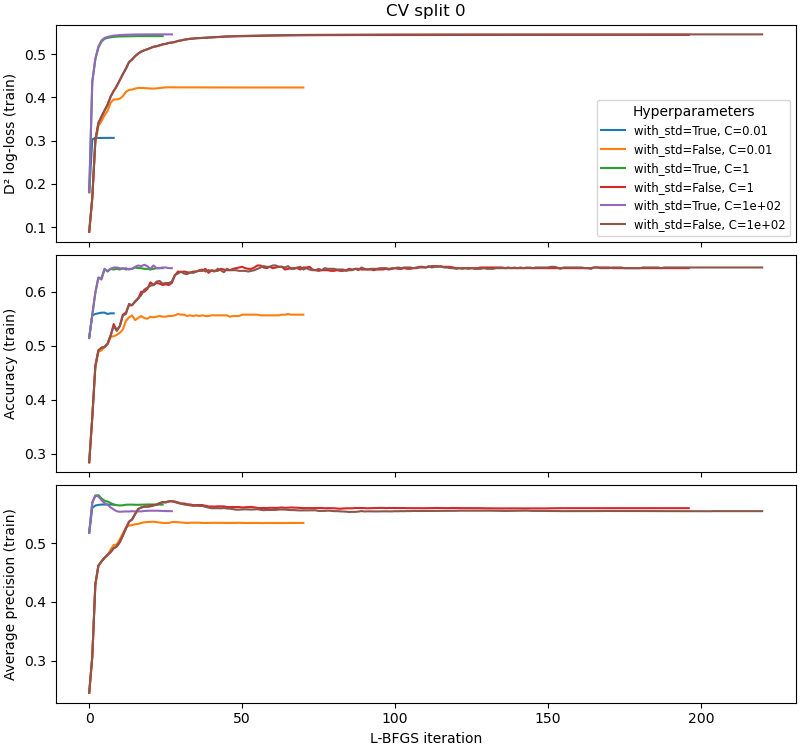
We define labels for plotting purposes and plot each metric separately.

cv_lbfgs_log["param_label"] = cv_lbfgs_log.apply(
    lambda row: (
        f"with_std={row['param_standardscaler__with_std']}, "
        f"C={row['param_logisticregression__C']:.2g}"
    ),
    axis=1,
)

metrics = {
    "d2_log_loss_score": "D² log-loss (train)",
    "accuracy": "Accuracy (train)",
    "average_precision": "Average precision (train)",
}
_, axes = plt.subplots(
    len(metrics),
    1,
    figsize=(8, 2.5 * len(metrics)),
    sharex=True,
    constrained_layout=True,
)
for idx, (metric, ylabel) in enumerate(metrics.items()):
    ax = axes[idx]
    for param_label, group in cv_lbfgs_log.groupby("param_label", sort=False):
        ax.plot(group["task_id"], group[metric], label=param_label)
    ax.set_ylabel(ylabel)
    if idx == 0:
        ax.set_title("CV split 0")
        ax.legend(title="Hyperparameters", fontsize="small")

_ = axes[-1].set_xlabel("L-BFGS iteration")

Analysis of the convergence of the logistic regression models#

D² log-loss convergence#

The D² log-loss scores generally improve monotonically for all models. This is expected because the logistic regression model is fitted by minimizing the (regularized) log-loss computed on the training set.

Accuracy fluctuations#

The accuracy score improves with the number of iterations, albeit with some local fluctuations. This is expected because accuracy is discontinuous and not directly optimized by the model. Instead the model minimizes the log-loss which is a smooth surrogate for the zero-one loss (and thus related to, but not directly optimized by, accuracy).

Regularization and scaling#

We also observe that the least regularized models (larger C values) tend to reach higher D² log-loss scores, and models trained on scaled features converge in much fewer iterations.

Furthermore, models trained with high regularization (lower C values) converge to a final D² log-loss value that depends on the regularization strength while this is not the case for models trained with low regularization: there is a strong coupling between the optimal regularization strength and the feature scaling.