Note
Go to the end to download the full example code or to run this example in your browser via JupyterLite or Binder.
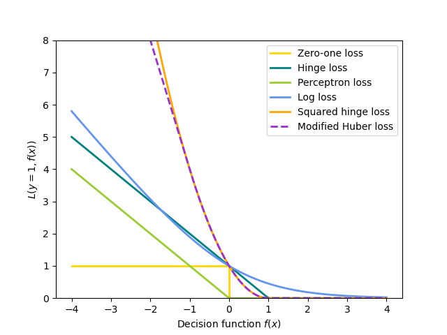
SGD: convex loss functions#
A plot that compares the various convex loss functions supported by
SGDClassifier .
# Authors: The scikit-learn developers
# SPDX-License-Identifier: BSD-3-Clause

import matplotlib.pyplot as plt
import numpy as np


def modified_huber_loss(y_true, y_pred):
    z = y_pred * y_true
    loss = -4 * z
    loss[z >= -1] = (1 - z[z >= -1]) ** 2
    loss[z >= 1.0] = 0
    return loss


xmin, xmax = -4, 4
xx = np.linspace(xmin, xmax, 100)
lw = 2
plt.plot([xmin, 0, 0, xmax], [1, 1, 0, 0], color="gold", lw=lw, label="Zero-one loss")
plt.plot(xx, np.where(xx < 1, 1 - xx, 0), color="teal", lw=lw, label="Hinge loss")
plt.plot(xx, -np.minimum(xx, 0), color="yellowgreen", lw=lw, label="Perceptron loss")
plt.plot(xx, np.log2(1 + np.exp(-xx)), color="cornflowerblue", lw=lw, label="Log loss")
plt.plot(
    xx,
    np.where(xx < 1, 1 - xx, 0) ** 2,
    color="orange",
    lw=lw,
    label="Squared hinge loss",
)
plt.plot(
    xx,
    modified_huber_loss(xx, 1),
    color="darkorchid",
    lw=lw,
    linestyle="--",
    label="Modified Huber loss",
)
plt.ylim((0, 8))
plt.legend(loc="upper right")
plt.xlabel(r"Decision function $f(x)$")
plt.ylabel("$L(y=1, f(x))$")
plt.show()
Total running time of the script: (0 minutes 0.084 seconds)
Related examples
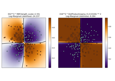
Illustration of Gaussian process classification (GPC) on the XOR dataset
Illustration of Gaussian process classification (GPC) on the XOR dataset
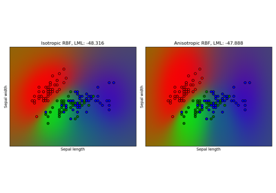
Gaussian process classification (GPC) on iris dataset
Gaussian process classification (GPC) on iris dataset
