Note
Go to the end to download the full example code or to run this example in your browser via JupyterLite or Binder.
Release Highlights for scikit-learn 0.24#
We are pleased to announce the release of scikit-learn 0.24! Many bug fixes and improvements were added, as well as some new key features. We detail below a few of the major features of this release. For an exhaustive list of all the changes, please refer to the release notes.
To install the latest version (with pip):
pip install --upgrade scikit-learn
or with conda:
conda install -c conda-forge scikit-learn
Successive Halving estimators for tuning hyper-parameters#
Successive Halving, a state of the art method, is now available to
explore the space of the parameters and identify their best combination.
HalvingGridSearchCV and
HalvingRandomSearchCV can be
used as drop-in replacement for
GridSearchCV and
RandomizedSearchCV.
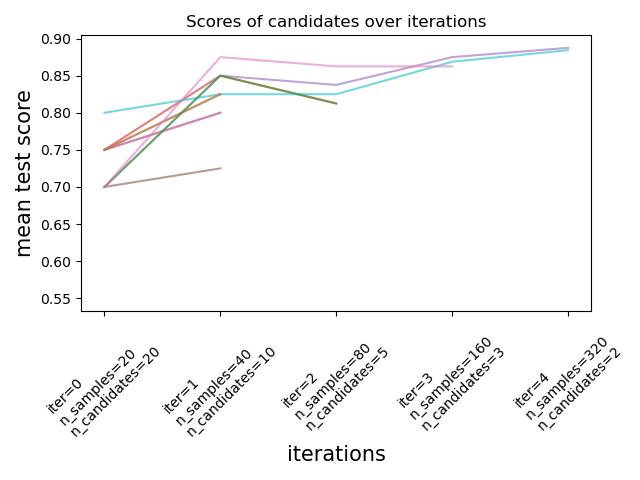
Successive Halving is an iterative selection process illustrated in the
figure below. The first iteration is run with a small amount of resources,
where the resource typically corresponds to the number of training samples,
but can also be an arbitrary integer parameter such as n_estimators in a
random forest. Only a subset of the parameter candidates are selected for the
next iteration, which will be run with an increasing amount of allocated
resources. Only a subset of candidates will last until the end of the
iteration process, and the best parameter candidate is the one that has the
highest score on the last iteration.
Read more in the User Guide (note: the Successive Halving estimators are still experimental).
import numpy as np
from scipy.stats import randint

from sklearn.datasets import make_classification
from sklearn.ensemble import RandomForestClassifier
from sklearn.experimental import enable_halving_search_cv  # noqa: F401
from sklearn.model_selection import HalvingRandomSearchCV

rng = np.random.RandomState(0)

X, y = make_classification(n_samples=700, random_state=rng)

clf = RandomForestClassifier(n_estimators=10, random_state=rng)

param_dist = {
    "max_depth": [3, None],
    "max_features": randint(1, 11),
    "min_samples_split": randint(2, 11),
    "bootstrap": [True, False],
    "criterion": ["gini", "entropy"],
}

rsh = HalvingRandomSearchCV(
    estimator=clf, param_distributions=param_dist, factor=2, random_state=rng
)
rsh.fit(X, y)
rsh.best_params_
{'bootstrap': True, 'criterion': 'gini', 'max_depth': None, 'max_features': 10, 'min_samples_split': 10}
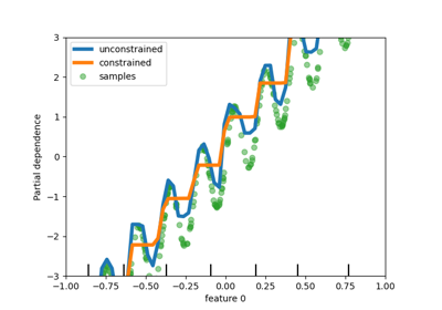
Native support for categorical features in HistGradientBoosting estimators#
HistGradientBoostingClassifier and
HistGradientBoostingRegressor now have native
support for categorical features: they can consider splits on non-ordered,
categorical data. Read more in the User Guide.

The plot shows that the new native support for categorical features leads to
fitting times that are comparable to models where the categories are treated
as ordered quantities, i.e. simply ordinal-encoded. Native support is also
more expressive than both one-hot encoding and ordinal encoding. However, to
use the new categorical_features parameter, it is still required to
preprocess the data within a pipeline as demonstrated in this example.
Improved performances of HistGradientBoosting estimators#
The memory footprint of ensemble.HistGradientBoostingRegressor and
ensemble.HistGradientBoostingClassifier has been significantly
improved during calls to fit. In addition, histogram initialization is now
done in parallel which results in slight speed improvements.
See more in the Benchmark page.
New self-training meta-estimator#
A new self-training implementation, based on Yarowski’s algorithm can now be used with any classifier that implements predict_proba. The sub-classifier will behave as a semi-supervised classifier, allowing it to learn from unlabeled data. Read more in the User guide.
import numpy as np

from sklearn import datasets
from sklearn.linear_model import LogisticRegression
from sklearn.semi_supervised import SelfTrainingClassifier

rng = np.random.RandomState(42)
iris = datasets.load_iris()
random_unlabeled_points = rng.rand(iris.target.shape[0]) < 0.3
iris.target[random_unlabeled_points] = -1
clf = LogisticRegression()
self_training_model = SelfTrainingClassifier(clf)
self_training_model.fit(iris.data, iris.target)
/home/circleci/project/sklearn/linear_model/_logistic.py:599: ConvergenceWarning: lbfgs failed to converge after 100 iteration(s) (status=1):
STOP: TOTAL NO. OF ITERATIONS REACHED LIMIT

Increase the number of iterations to improve the convergence (max_iter=100).
You might also want to scale the data as shown in:
    https://scikit-learn.org/stable/modules/preprocessing.html
Please also refer to the documentation for alternative solver options:
    https://scikit-learn.org/stable/modules/linear_model.html#logistic-regression
  n_iter_i = _check_optimize_result(
New SequentialFeatureSelector transformer#
A new iterative transformer to select features is available:
SequentialFeatureSelector.
Sequential Feature Selection can add features one at a time (forward
selection) or remove features from the list of the available features
(backward selection), based on a cross-validated score maximization.
See the User Guide.
from sklearn.datasets import load_iris
from sklearn.feature_selection import SequentialFeatureSelector
from sklearn.neighbors import KNeighborsClassifier

X, y = load_iris(return_X_y=True, as_frame=True)
feature_names = X.columns
knn = KNeighborsClassifier(n_neighbors=3)
sfs = SequentialFeatureSelector(knn, n_features_to_select=2)
sfs.fit(X, y)
print(
    "Features selected by forward sequential selection: "
    f"{feature_names[sfs.get_support()].tolist()}"
)
Features selected by forward sequential selection: ['sepal length (cm)', 'petal width (cm)']
New PolynomialCountSketch kernel approximation function#
The new PolynomialCountSketch
approximates a polynomial expansion of a feature space when used with linear
models, but uses much less memory than
PolynomialFeatures.
from sklearn.datasets import fetch_covtype
from sklearn.kernel_approximation import PolynomialCountSketch
from sklearn.linear_model import LogisticRegression
from sklearn.model_selection import train_test_split
from sklearn.pipeline import make_pipeline
from sklearn.preprocessing import MinMaxScaler

X, y = fetch_covtype(return_X_y=True)
pipe = make_pipeline(
    MinMaxScaler(),
    PolynomialCountSketch(degree=2, n_components=300),
    LogisticRegression(max_iter=1000),
)
X_train, X_test, y_train, y_test = train_test_split(
    X, y, train_size=5000, test_size=10000, random_state=42
)
pipe.fit(X_train, y_train).score(X_test, y_test)
0.7343
For comparison, here is the score of a linear baseline for the same data:
linear_baseline = make_pipeline(MinMaxScaler(), LogisticRegression(max_iter=1000))
linear_baseline.fit(X_train, y_train).score(X_test, y_test)
0.7135
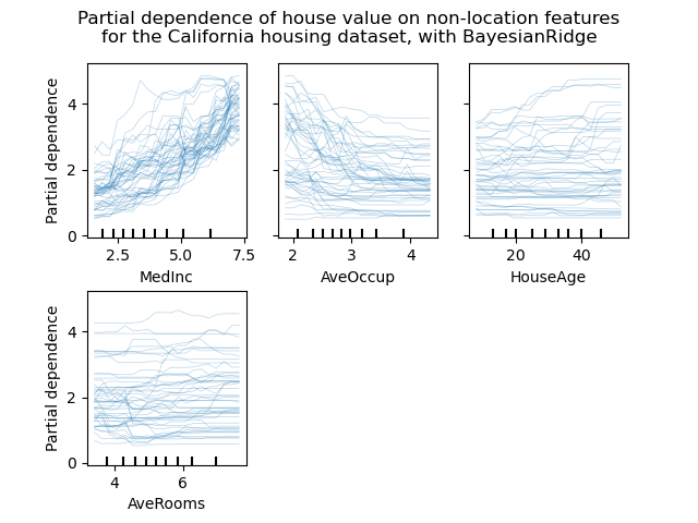
Individual Conditional Expectation plots#
A new kind of partial dependence plot is available: the Individual Conditional Expectation (ICE) plot. ICE plots visualize the dependence of the prediction on a feature for each sample separately, with one line per sample. See the User Guide
from sklearn.datasets import fetch_california_housing
from sklearn.ensemble import RandomForestRegressor

# from sklearn.inspection import plot_partial_dependence
from sklearn.inspection import PartialDependenceDisplay

X, y = fetch_california_housing(return_X_y=True, as_frame=True)
features = ["MedInc", "AveOccup", "HouseAge", "AveRooms"]
est = RandomForestRegressor(n_estimators=10)
est.fit(X, y)

# plot_partial_dependence has been removed in version 1.2. From 1.2, use
# PartialDependenceDisplay instead.
# display = plot_partial_dependence(
display = PartialDependenceDisplay.from_estimator(
    est,
    X,
    features,
    kind="individual",
    subsample=50,
    n_jobs=3,
    grid_resolution=20,
    random_state=0,
)
display.figure_.suptitle(
    "Partial dependence of house value on non-location features\n"
    "for the California housing dataset, with BayesianRidge"
)
display.figure_.subplots_adjust(hspace=0.3)
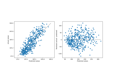
New Poisson splitting criterion for DecisionTreeRegressor#
The integration of Poisson regression estimation continues from version 0.23.
DecisionTreeRegressor now supports a new 'poisson'
splitting criterion. Setting criterion="poisson" might be a good choice
if your target is a count or a frequency.
import numpy as np

from sklearn.model_selection import train_test_split
from sklearn.tree import DecisionTreeRegressor

n_samples, n_features = 1000, 20
rng = np.random.RandomState(0)
X = rng.randn(n_samples, n_features)
# positive integer target correlated with X[:, 5] with many zeros:
y = rng.poisson(lam=np.exp(X[:, 5]) / 2)
X_train, X_test, y_train, y_test = train_test_split(X, y, random_state=rng)
regressor = DecisionTreeRegressor(criterion="poisson", random_state=0)
regressor.fit(X_train, y_train)
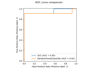
New documentation improvements#
New examples and documentation pages have been added, in a continuous effort to improve the understanding of machine learning practices:
a new section about common pitfalls and recommended practices,
an example illustrating how to statistically compare the performance of models evaluated using
GridSearchCV,an example on how to interpret coefficients of linear models,
an example comparing Principal Component Regression and Partial Least Squares.
Total running time of the script: (0 minutes 14.868 seconds)
Related examples