Note
Go to the end to download the full example code or to run this example in your browser via JupyterLite or Binder.
Effect of model regularization on training and test error#
In this example, we evaluate the impact of the regularization parameter in a
linear model called ElasticNet. To carry out this
evaluation, we use a validation curve using
ValidationCurveDisplay. This curve shows the
training and test scores of the model for different values of the regularization
parameter.
Once we identify the optimal regularization parameter, we compare the true and estimated coefficients of the model to determine if the model is able to recover the coefficients from the noisy input data.
# Authors: The scikit-learn developers
# SPDX-License-Identifier: BSD-3-Clause
Generate sample data#
We generate a regression dataset that contains many features relative to the number of samples. However, only 10% of the features are informative. In this context, linear models exposing L1 penalization are commonly used to recover a sparse set of coefficients.
from sklearn.datasets import make_regression
from sklearn.model_selection import train_test_split

n_samples_train, n_samples_test, n_features = 150, 300, 500
X, y, true_coef = make_regression(
    n_samples=n_samples_train + n_samples_test,
    n_features=n_features,
    n_informative=50,
    shuffle=False,
    noise=1.0,
    coef=True,
    random_state=42,
)
X_train, X_test, y_train, y_test = train_test_split(
    X, y, train_size=n_samples_train, test_size=n_samples_test, shuffle=False
)
Model definition#
Here, we do not use a model that only exposes an L1 penalty. Instead, we use
an ElasticNet model that exposes both L1 and L2
penalties.
We fix the l1_ratio parameter such that the solution found by the model is still
sparse. Therefore, this type of model tries to find a sparse solution but at the same
time also tries to shrink all coefficients towards zero.
In addition, we force the coefficients of the model to be positive since we know that
make_regression generates a response with a positive signal. So we use this
pre-knowledge to get a better model.
from sklearn.linear_model import ElasticNet

enet = ElasticNet(l1_ratio=0.9, positive=True, max_iter=10_000)
Evaluate the impact of the regularization parameter#
To evaluate the impact of the regularization parameter, we use a validation curve. This curve shows the training and test scores of the model for different values of the regularization parameter.
The regularization alpha is a parameter applied to the coefficients of the model:
when it tends to zero, no regularization is applied and the model tries to fit the
training data with the least amount of error. However, it leads to overfitting when
features are noisy. When alpha increases, the model coefficients are constrained,
and thus the model cannot fit the training data as closely, avoiding overfitting.
However, if too much regularization is applied, the model underfits the data and
is not able to properly capture the signal.
The validation curve helps in finding a good trade-off between both extremes: the
model is not regularized and thus flexible enough to fit the signal, but not too
flexible to overfit. The ValidationCurveDisplay
allows us to display the training and validation scores across a range of alpha
values.
import numpy as np

from sklearn.model_selection import ValidationCurveDisplay

alphas = np.logspace(-5, 1, 60)
disp = ValidationCurveDisplay.from_estimator(
    enet,
    X_train,
    y_train,
    param_name="alpha",
    param_range=alphas,
    scoring="r2",
    n_jobs=2,
    score_type="both",
)
disp.ax_.set(
    title=r"Validation Curve for ElasticNet (R$^2$ Score)",
    xlabel=r"alpha (regularization strength)",
    ylabel="R$^2$ Score",
)

test_scores_mean = disp.test_scores.mean(axis=1)
idx_avg_max_test_score = np.argmax(test_scores_mean)
disp.ax_.vlines(
    alphas[idx_avg_max_test_score],
    disp.ax_.get_ylim()[0],
    test_scores_mean[idx_avg_max_test_score],
    color="k",
    linewidth=2,
    linestyle="--",
    label=f"Optimum on test\n$\\alpha$ = {alphas[idx_avg_max_test_score]:.2e}",
)
_ = disp.ax_.legend(loc="lower right")
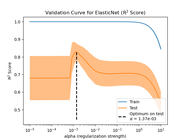
To find the optimal regularization parameter, we can select the value of alpha
that maximizes the validation score.
Coefficients comparison#
Now that we have identified the optimal regularization parameter, we can compare the true coefficients and the estimated coefficients.
First, let’s set the regularization parameter to the optimal value and fit the model on the training data. In addition, we’ll show the test score for this model.
enet.set_params(alpha=alphas[idx_avg_max_test_score]).fit(X_train, y_train)
print(
    f"Test score: {enet.score(X_test, y_test):.3f}",
)
Test score: 0.884
Now, we plot the true coefficients and the estimated coefficients.
import matplotlib.pyplot as plt

fig, axs = plt.subplots(ncols=2, figsize=(12, 6), sharex=True, sharey=True)
for ax, coef, title in zip(axs, [true_coef, enet.coef_], ["True", "Model"]):
    ax.stem(coef)
    ax.set(
        title=f"{title} Coefficients",
        xlabel="Feature Index",
        ylabel="Coefficient Value",
    )
fig.suptitle(
    "Comparison of the coefficients of the true generative model and \n"
    "the estimated elastic net coefficients"
)

plt.show()
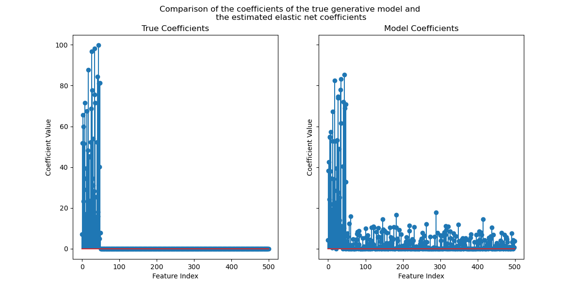
While the original coefficients are sparse, the estimated coefficients are not
as sparse. The reason is that we fixed the l1_ratio parameter to 0.9. We could
force the model to get a sparser solution by increasing the l1_ratio parameter.
However, we observed that for the estimated coefficients that are close to zero in the true generative model, our model shrinks them towards zero. So we don’t recover the true coefficients, but we get a sensible outcome in line with the performance obtained on the test set.
Total running time of the script: (0 minutes 7.107 seconds)
Related examples
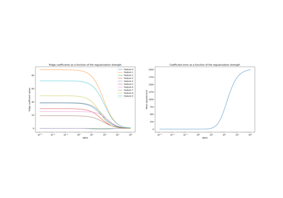
Ridge coefficients as a function of the L2 Regularization
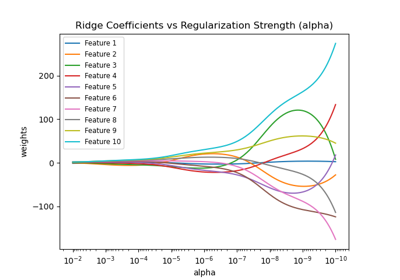
Plot Ridge coefficients as a function of the regularization