Note
Go to the end to download the full example code or to run this example in your browser via JupyterLite or Binder.
Robust vs Empirical covariance estimate#
The usual covariance maximum likelihood estimate is very sensitive to the presence of outliers in the data set. In such a case, it would be better to use a robust estimator of covariance to guarantee that the estimation is resistant to “erroneous” observations in the data set. [1], [2]
Minimum Covariance Determinant Estimator#
The Minimum Covariance Determinant estimator is a robust, high-breakdown point (i.e. it can be used to estimate the covariance matrix of highly contaminated datasets, up to \(\frac{n_\text{samples} - n_\text{features}-1}{2}\) outliers) estimator of covariance. The idea is to find \(\frac{n_\text{samples} + n_\text{features}+1}{2}\) observations whose empirical covariance has the smallest determinant, yielding a “pure” subset of observations from which to compute standards estimates of location and covariance. After a correction step aiming at compensating the fact that the estimates were learned from only a portion of the initial data, we end up with robust estimates of the data set location and covariance.
The Minimum Covariance Determinant estimator (MCD) has been introduced by P.J.Rousseuw in [3].
Evaluation#
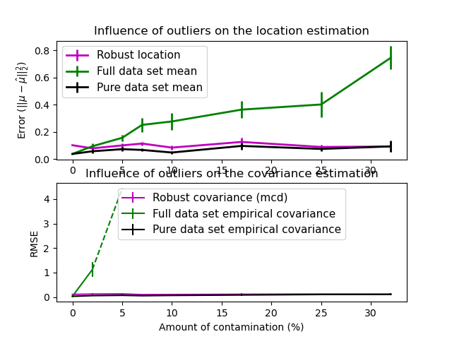
In this example, we compare the estimation errors that are made when using various types of location and covariance estimates on contaminated Gaussian distributed data sets:
The mean and the empirical covariance of the full dataset, which break down as soon as there are outliers in the data set
The robust MCD, that has a low error provided \(n_\text{samples} > 5n_\text{features}\)
The mean and the empirical covariance of the observations that are known to be good ones. This can be considered as a “perfect” MCD estimation, so one can trust our implementation by comparing to this case.
References#
# Authors: The scikit-learn developers
# SPDX-License-Identifier: BSD-3-Clause

import matplotlib.font_manager
import matplotlib.pyplot as plt
import numpy as np

from sklearn.covariance import EmpiricalCovariance, MinCovDet

# example settings
n_samples = 80
n_features = 5
repeat = 10

range_n_outliers = np.concatenate(
    (
        np.linspace(0, n_samples / 8, 5),
        np.linspace(n_samples / 8, n_samples / 2, 5)[1:-1],
    )
).astype(int)

# definition of arrays to store results
err_loc_mcd = np.zeros((range_n_outliers.size, repeat))
err_cov_mcd = np.zeros((range_n_outliers.size, repeat))
err_loc_emp_full = np.zeros((range_n_outliers.size, repeat))
err_cov_emp_full = np.zeros((range_n_outliers.size, repeat))
err_loc_emp_pure = np.zeros((range_n_outliers.size, repeat))
err_cov_emp_pure = np.zeros((range_n_outliers.size, repeat))

# computation
for i, n_outliers in enumerate(range_n_outliers):
    for j in range(repeat):
        rng = np.random.RandomState(i * j)

        # generate data
        X = rng.randn(n_samples, n_features)
        # add some outliers
        outliers_index = rng.permutation(n_samples)[:n_outliers]
        outliers_offset = 10.0 * (
            np.random.randint(2, size=(n_outliers, n_features)) - 0.5
        )
        X[outliers_index] += outliers_offset
        inliers_mask = np.ones(n_samples).astype(bool)
        inliers_mask[outliers_index] = False

        # fit a Minimum Covariance Determinant (MCD) robust estimator to data
        mcd = MinCovDet().fit(X)
        # compare raw robust estimates with the true location and covariance
        err_loc_mcd[i, j] = np.sum(mcd.location_**2)
        err_cov_mcd[i, j] = mcd.error_norm(np.eye(n_features))

        # compare estimators learned from the full data set with true
        # parameters
        err_loc_emp_full[i, j] = np.sum(X.mean(0) ** 2)
        err_cov_emp_full[i, j] = (
            EmpiricalCovariance().fit(X).error_norm(np.eye(n_features))
        )

        # compare with an empirical covariance learned from a pure data set
        # (i.e. "perfect" mcd)
        pure_X = X[inliers_mask]
        pure_location = pure_X.mean(0)
        pure_emp_cov = EmpiricalCovariance().fit(pure_X)
        err_loc_emp_pure[i, j] = np.sum(pure_location**2)
        err_cov_emp_pure[i, j] = pure_emp_cov.error_norm(np.eye(n_features))

# Display results
font_prop = matplotlib.font_manager.FontProperties(size=11)
plt.subplot(2, 1, 1)
lw = 2
plt.errorbar(
    range_n_outliers,
    err_loc_mcd.mean(1),
    yerr=err_loc_mcd.std(1) / np.sqrt(repeat),
    label="Robust location",
    lw=lw,
    color="m",
)
plt.errorbar(
    range_n_outliers,
    err_loc_emp_full.mean(1),
    yerr=err_loc_emp_full.std(1) / np.sqrt(repeat),
    label="Full data set mean",
    lw=lw,
    color="green",
)
plt.errorbar(
    range_n_outliers,
    err_loc_emp_pure.mean(1),
    yerr=err_loc_emp_pure.std(1) / np.sqrt(repeat),
    label="Pure data set mean",
    lw=lw,
    color="black",
)
plt.title("Influence of outliers on the location estimation")
plt.ylabel(r"Error ($||\mu - \hat{\mu}||_2^2$)")
plt.legend(loc="upper left", prop=font_prop)

plt.subplot(2, 1, 2)
x_size = range_n_outliers.size
plt.errorbar(
    range_n_outliers,
    err_cov_mcd.mean(1),
    yerr=err_cov_mcd.std(1),
    label="Robust covariance (mcd)",
    color="m",
)
plt.errorbar(
    range_n_outliers[: (x_size // 5 + 1)],
    err_cov_emp_full.mean(1)[: (x_size // 5 + 1)],
    yerr=err_cov_emp_full.std(1)[: (x_size // 5 + 1)],
    label="Full data set empirical covariance",
    color="green",
)
plt.plot(
    range_n_outliers[(x_size // 5) : (x_size // 2 - 1)],
    err_cov_emp_full.mean(1)[(x_size // 5) : (x_size // 2 - 1)],
    color="green",
    ls="--",
)
plt.errorbar(
    range_n_outliers,
    err_cov_emp_pure.mean(1),
    yerr=err_cov_emp_pure.std(1),
    label="Pure data set empirical covariance",
    color="black",
)
plt.title("Influence of outliers on the covariance estimation")
plt.xlabel("Amount of contamination (%)")
plt.ylabel("RMSE")
plt.legend(loc="center", prop=font_prop)

plt.tight_layout()
plt.show()
Total running time of the script: (0 minutes 3.185 seconds)
Related examples
Robust covariance estimation and Mahalanobis distances relevance
Linear and Quadratic Discriminant Analysis with covariance ellipsoid
