Note
Go to the end to download the full example code or to run this example in your browser via JupyterLite or Binder.
Hashing feature transformation using Totally Random Trees#
RandomTreesEmbedding provides a way to map data to a very high-dimensional, sparse representation, which might be beneficial for classification. The mapping is completely unsupervised and very efficient.
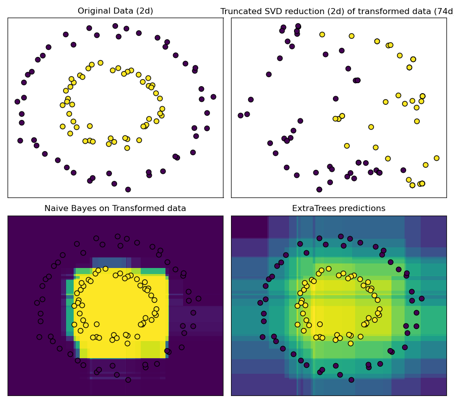
This example visualizes the partitions given by several trees and shows how the transformation can also be used for non-linear dimensionality reduction or non-linear classification.
Points that are neighboring often share the same leaf of a tree and therefore share large parts of their hashed representation. This allows to separate two concentric circles simply based on the principal components of the transformed data with truncated SVD.
In high-dimensional spaces, linear classifiers often achieve excellent accuracy. For sparse binary data, BernoulliNB is particularly well-suited. The bottom row compares the decision boundary obtained by BernoulliNB in the transformed space with an ExtraTreesClassifier forests learned on the original data.
# Authors: The scikit-learn developers
# SPDX-License-Identifier: BSD-3-Clause

import matplotlib.pyplot as plt
import numpy as np

from sklearn.datasets import make_circles
from sklearn.decomposition import TruncatedSVD
from sklearn.ensemble import ExtraTreesClassifier, RandomTreesEmbedding
from sklearn.naive_bayes import BernoulliNB

# make a synthetic dataset
X, y = make_circles(factor=0.5, random_state=0, noise=0.05)

# use RandomTreesEmbedding to transform data
hasher = RandomTreesEmbedding(n_estimators=10, random_state=0, max_depth=3)
X_transformed = hasher.fit_transform(X)

# Visualize result after dimensionality reduction using truncated SVD
svd = TruncatedSVD(n_components=2)
X_reduced = svd.fit_transform(X_transformed)

# Learn a Naive Bayes classifier on the transformed data
nb = BernoulliNB()
nb.fit(X_transformed, y)


# Learn an ExtraTreesClassifier for comparison
trees = ExtraTreesClassifier(max_depth=3, n_estimators=10, random_state=0)
trees.fit(X, y)


# scatter plot of original and reduced data
fig = plt.figure(figsize=(9, 8))

ax = plt.subplot(221)
ax.scatter(X[:, 0], X[:, 1], c=y, s=50, edgecolor="k")
ax.set_title("Original Data (2d)")
ax.set_xticks(())
ax.set_yticks(())

ax = plt.subplot(222)
ax.scatter(X_reduced[:, 0], X_reduced[:, 1], c=y, s=50, edgecolor="k")
ax.set_title(
    "Truncated SVD reduction (2d) of transformed data (%dd)" % X_transformed.shape[1]
)
ax.set_xticks(())
ax.set_yticks(())

# Plot the decision in original space. For that, we will assign a color
# to each point in the mesh [x_min, x_max]x[y_min, y_max].
h = 0.01
x_min, x_max = X[:, 0].min() - 0.5, X[:, 0].max() + 0.5
y_min, y_max = X[:, 1].min() - 0.5, X[:, 1].max() + 0.5
xx, yy = np.meshgrid(np.arange(x_min, x_max, h), np.arange(y_min, y_max, h))

# transform grid using RandomTreesEmbedding
transformed_grid = hasher.transform(np.c_[xx.ravel(), yy.ravel()])
y_grid_pred = nb.predict_proba(transformed_grid)[:, 1]

ax = plt.subplot(223)
ax.set_title("Naive Bayes on Transformed data")
ax.pcolormesh(xx, yy, y_grid_pred.reshape(xx.shape))
ax.scatter(X[:, 0], X[:, 1], c=y, s=50, edgecolor="k")
ax.set_ylim(-1.4, 1.4)
ax.set_xlim(-1.4, 1.4)
ax.set_xticks(())
ax.set_yticks(())

# transform grid using ExtraTreesClassifier
y_grid_pred = trees.predict_proba(np.c_[xx.ravel(), yy.ravel()])[:, 1]

ax = plt.subplot(224)
ax.set_title("ExtraTrees predictions")
ax.pcolormesh(xx, yy, y_grid_pred.reshape(xx.shape))
ax.scatter(X[:, 0], X[:, 1], c=y, s=50, edgecolor="k")
ax.set_ylim(-1.4, 1.4)
ax.set_xlim(-1.4, 1.4)
ax.set_xticks(())
ax.set_yticks(())

plt.tight_layout()
plt.show()
Total running time of the script: (0 minutes 0.452 seconds)
Related examples
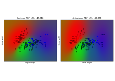
Gaussian process classification (GPC) on iris dataset