Note
Go to the end to download the full example code or to run this example in your browser via JupyterLite or Binder.
Swiss Roll And Swiss-Hole Reduction#
This notebook seeks to compare two popular non-linear dimensionality techniques, T-distributed Stochastic Neighbor Embedding (t-SNE) and Locally Linear Embedding (LLE), on the classic Swiss Roll dataset. Then, we will explore how they both deal with the addition of a hole in the data.
# Authors: The scikit-learn developers
# SPDX-License-Identifier: BSD-3-Clause
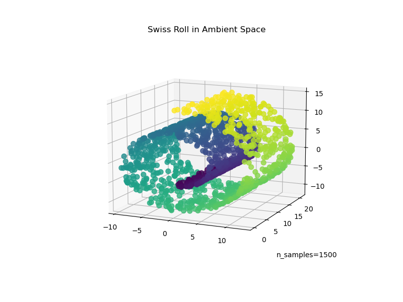
Swiss Roll#
We start by generating the Swiss Roll dataset.
import matplotlib.pyplot as plt

from sklearn import datasets, manifold

sr_points, sr_color = datasets.make_swiss_roll(n_samples=1500, random_state=0)
Now, let’s take a look at our data:
fig = plt.figure(figsize=(8, 6))
ax = fig.add_subplot(111, projection="3d")
fig.add_axes(ax)
ax.scatter(
    sr_points[:, 0], sr_points[:, 1], sr_points[:, 2], c=sr_color, s=50, alpha=0.8
)
ax.set_title("Swiss Roll in Ambient Space")
ax.view_init(azim=-66, elev=12)
_ = ax.text2D(0.8, 0.05, s="n_samples=1500", transform=ax.transAxes)
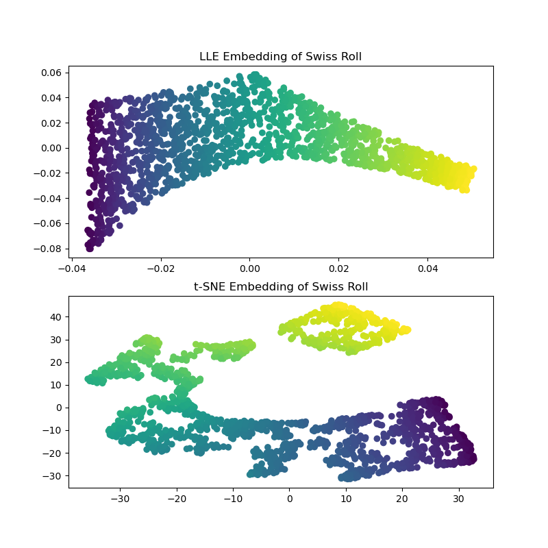
Computing the LLE and t-SNE embeddings, we find that LLE seems to unroll the Swiss Roll pretty effectively. t-SNE on the other hand, is able to preserve the general structure of the data, but, poorly represents the continuous nature of our original data. Instead, it seems to unnecessarily clump sections of points together.
sr_lle, sr_err = manifold.locally_linear_embedding(
    sr_points, n_neighbors=12, n_components=2
)

sr_tsne = manifold.TSNE(n_components=2, perplexity=40, random_state=0).fit_transform(
    sr_points
)

fig, axs = plt.subplots(figsize=(8, 8), nrows=2)
axs[0].scatter(sr_lle[:, 0], sr_lle[:, 1], c=sr_color)
axs[0].set_title("LLE Embedding of Swiss Roll")
axs[1].scatter(sr_tsne[:, 0], sr_tsne[:, 1], c=sr_color)
_ = axs[1].set_title("t-SNE Embedding of Swiss Roll")
Note
LLE seems to be stretching the points from the center (purple) of the swiss roll. However, we observe that this is simply a byproduct of how the data was generated. There is a higher density of points near the center of the roll, which ultimately affects how LLE reconstructs the data in a lower dimension.
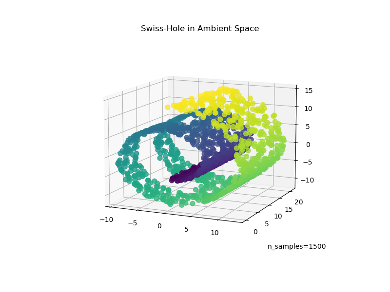
Swiss-Hole#
Now let’s take a look at how both algorithms deal with us adding a hole to the data. First, we generate the Swiss-Hole dataset and plot it:
sh_points, sh_color = datasets.make_swiss_roll(
    n_samples=1500, hole=True, random_state=0
)

fig = plt.figure(figsize=(8, 6))
ax = fig.add_subplot(111, projection="3d")
fig.add_axes(ax)
ax.scatter(
    sh_points[:, 0], sh_points[:, 1], sh_points[:, 2], c=sh_color, s=50, alpha=0.8
)
ax.set_title("Swiss-Hole in Ambient Space")
ax.view_init(azim=-66, elev=12)
_ = ax.text2D(0.8, 0.05, s="n_samples=1500", transform=ax.transAxes)
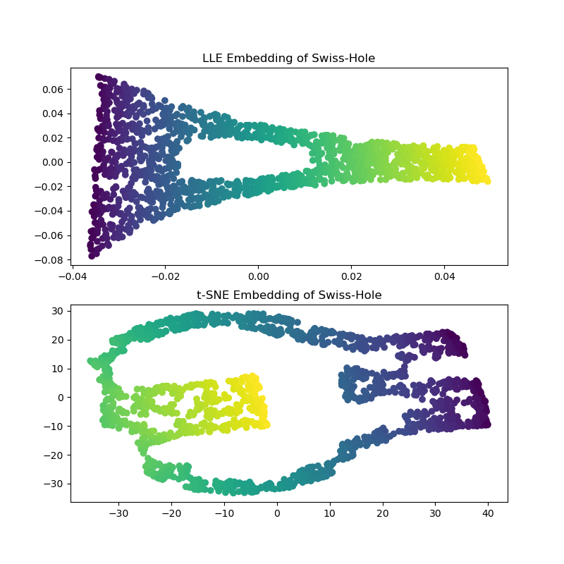
Computing the LLE and t-SNE embeddings, we obtain similar results to the Swiss Roll. LLE very capably unrolls the data and even preserves the hole. t-SNE, again seems to clump sections of points together, but, we note that it preserves the general topology of the original data.
sh_lle, sh_err = manifold.locally_linear_embedding(
    sh_points, n_neighbors=12, n_components=2
)

sh_tsne = manifold.TSNE(
    n_components=2, perplexity=40, init="random", random_state=0
).fit_transform(sh_points)

fig, axs = plt.subplots(figsize=(8, 8), nrows=2)
axs[0].scatter(sh_lle[:, 0], sh_lle[:, 1], c=sh_color)
axs[0].set_title("LLE Embedding of Swiss-Hole")
axs[1].scatter(sh_tsne[:, 0], sh_tsne[:, 1], c=sh_color)
_ = axs[1].set_title("t-SNE Embedding of Swiss-Hole")
Concluding remarks#
We note that t-SNE benefits from testing more combinations of parameters. Better results could probably have been obtained by better tuning these parameters.
We observe that, as seen in the “Manifold learning on handwritten digits” example, t-SNE generally performs better than LLE on real world data.
Total running time of the script: (0 minutes 18.067 seconds)
Related examples
Manifold learning on handwritten digits: Locally Linear Embedding, Isomap…
Hierarchical clustering with and without structure
