Note
Go to the end to download the full example code or to run this example in your browser via JupyterLite or Binder.
Release Highlights for scikit-learn 0.22#
We are pleased to announce the release of scikit-learn 0.22, which comes with many bug fixes and new features! We detail below a few of the major features of this release. For an exhaustive list of all the changes, please refer to the release notes.
To install the latest version (with pip):
pip install --upgrade scikit-learn
or with conda:
conda install -c conda-forge scikit-learn
# Authors: The scikit-learn developers
# SPDX-License-Identifier: BSD-3-Clause
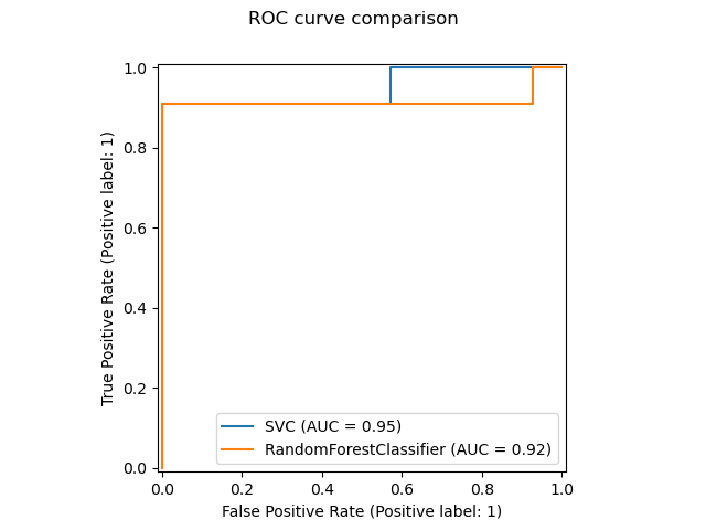
New plotting API#
A new plotting API is available for creating visualizations. This new API
allows for quickly adjusting the visuals of a plot without involving any
recomputation. It is also possible to add different plots to the same
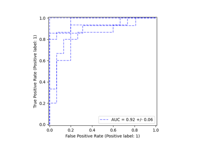
figure. The following example illustrates plot_roc_curve,
but other plots utilities are supported like
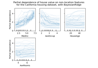
plot_partial_dependence,
plot_precision_recall_curve, and
plot_confusion_matrix. Read more about this new API in the
User Guide.
import matplotlib
import matplotlib.pyplot as plt

from sklearn.datasets import make_classification
from sklearn.ensemble import RandomForestClassifier

# from sklearn.metrics import plot_roc_curve
from sklearn.metrics import RocCurveDisplay
from sklearn.model_selection import train_test_split
from sklearn.svm import SVC
from sklearn.utils.fixes import parse_version

X, y = make_classification(random_state=0)
X_train, X_test, y_train, y_test = train_test_split(X, y, random_state=42)

svc = SVC(random_state=42)
svc.fit(X_train, y_train)
rfc = RandomForestClassifier(random_state=42)
rfc.fit(X_train, y_train)

# plot_roc_curve has been removed in version 1.2. From 1.2, use RocCurveDisplay instead.
# svc_disp = plot_roc_curve(svc, X_test, y_test)
# rfc_disp = plot_roc_curve(rfc, X_test, y_test, ax=svc_disp.ax_)
svc_disp = RocCurveDisplay.from_estimator(svc, X_test, y_test)
rfc_disp = RocCurveDisplay.from_estimator(rfc, X_test, y_test, ax=svc_disp.ax_)
rfc_disp.figure_.suptitle("ROC curve comparison")

plt.show()
Stacking Classifier and Regressor#
StackingClassifier and
StackingRegressor
allow you to have a stack of estimators with a final classifier or
a regressor.
Stacked generalization consists in stacking the output of individual
estimators and use a classifier to compute the final prediction. Stacking
allows to use the strength of each individual estimator by using their output
as input of a final estimator.
Base estimators are fitted on the full X while
the final estimator is trained using cross-validated predictions of the
base estimators using cross_val_predict.
Read more in the User Guide.
from sklearn.datasets import load_iris
from sklearn.ensemble import StackingClassifier
from sklearn.linear_model import LogisticRegression
from sklearn.model_selection import train_test_split
from sklearn.pipeline import make_pipeline
from sklearn.preprocessing import StandardScaler
from sklearn.svm import LinearSVC

X, y = load_iris(return_X_y=True)
estimators = [
    ("rf", RandomForestClassifier(n_estimators=10, random_state=42)),
    ("svr", make_pipeline(StandardScaler(), LinearSVC(dual="auto", random_state=42))),
]
clf = StackingClassifier(estimators=estimators, final_estimator=LogisticRegression())
X_train, X_test, y_train, y_test = train_test_split(X, y, stratify=y, random_state=42)
clf.fit(X_train, y_train).score(X_test, y_test)
0.9473684210526315
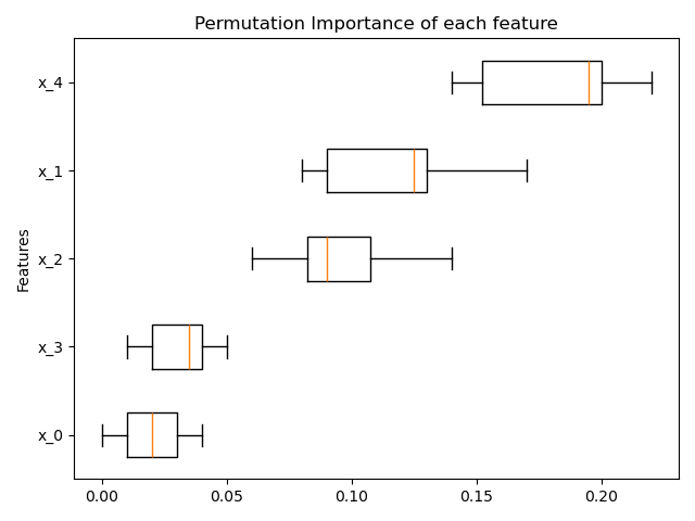
Permutation-based feature importance#
The inspection.permutation_importance can be used to get an
estimate of the importance of each feature, for any fitted estimator:
import matplotlib.pyplot as plt
import numpy as np

from sklearn.datasets import make_classification
from sklearn.ensemble import RandomForestClassifier
from sklearn.inspection import permutation_importance

X, y = make_classification(random_state=0, n_features=5, n_informative=3)
feature_names = np.array([f"x_{i}" for i in range(X.shape[1])])

rf = RandomForestClassifier(random_state=0).fit(X, y)
result = permutation_importance(rf, X, y, n_repeats=10, random_state=0, n_jobs=2)

fig, ax = plt.subplots()
sorted_idx = result.importances_mean.argsort()

# `labels` argument in boxplot is deprecated in matplotlib 3.9 and has been
# renamed to `tick_labels`. The following code handles this, but as a
# scikit-learn user you probably can write simpler code by using `labels=...`
# (matplotlib < 3.9) or `tick_labels=...` (matplotlib >= 3.9).
tick_labels_parameter_name = (
    "tick_labels"
    if parse_version(matplotlib.__version__) >= parse_version("3.9")
    else "labels"
)
tick_labels_dict = {tick_labels_parameter_name: feature_names[sorted_idx]}
ax.boxplot(result.importances[sorted_idx].T, vert=False, **tick_labels_dict)
ax.set_title("Permutation Importance of each feature")
ax.set_ylabel("Features")
fig.tight_layout()
plt.show()
Native support for missing values for gradient boosting#
The ensemble.HistGradientBoostingClassifier
and ensemble.HistGradientBoostingRegressor now have native
support for missing values (NaNs). This means that there is no need for
imputing data when training or predicting.
from sklearn.ensemble import HistGradientBoostingClassifier

X = np.array([0, 1, 2, np.nan]).reshape(-1, 1)
y = [0, 0, 1, 1]

gbdt = HistGradientBoostingClassifier(min_samples_leaf=1).fit(X, y)
print(gbdt.predict(X))
[0 0 1 1]
Precomputed sparse nearest neighbors graph#
Most estimators based on nearest neighbors graphs now accept precomputed
sparse graphs as input, to reuse the same graph for multiple estimator fits.
To use this feature in a pipeline, one can use the memory parameter, along
with one of the two new transformers,
neighbors.KNeighborsTransformer and
neighbors.RadiusNeighborsTransformer. The precomputation
can also be performed by custom estimators to use alternative
implementations, such as approximate nearest neighbors methods.
See more details in the User Guide.
from tempfile import TemporaryDirectory

from sklearn.manifold import Isomap
from sklearn.neighbors import KNeighborsTransformer
from sklearn.pipeline import make_pipeline

X, y = make_classification(random_state=0)

with TemporaryDirectory(prefix="sklearn_cache_") as tmpdir:
    estimator = make_pipeline(
        KNeighborsTransformer(n_neighbors=10, mode="distance"),
        Isomap(n_neighbors=10, metric="precomputed"),
        memory=tmpdir,
    )
    estimator.fit(X)

    # We can decrease the number of neighbors and the graph will not be
    # recomputed.
    estimator.set_params(isomap__n_neighbors=5)
    estimator.fit(X)
KNN Based Imputation#
We now support imputation for completing missing values using k-Nearest Neighbors.
Each sample’s missing values are imputed using the mean value from
n_neighbors nearest neighbors found in the training set. Two samples are
close if the features that neither is missing are close.
By default, a euclidean distance metric
that supports missing values,
nan_euclidean_distances, is used to find the nearest
neighbors.
Read more in the User Guide.
from sklearn.impute import KNNImputer

X = [[1, 2, np.nan], [3, 4, 3], [np.nan, 6, 5], [8, 8, 7]]
imputer = KNNImputer(n_neighbors=2)
print(imputer.fit_transform(X))
[[1.  2.  4. ]
 [3.  4.  3. ]
 [5.5 6.  5. ]
 [8.  8.  7. ]]
Tree pruning#
It is now possible to prune most tree-based estimators once the trees are built. The pruning is based on minimal cost-complexity. Read more in the User Guide for details.
X, y = make_classification(random_state=0)

rf = RandomForestClassifier(random_state=0, ccp_alpha=0).fit(X, y)
print(
    "Average number of nodes without pruning {:.1f}".format(
        np.mean([e.tree_.node_count for e in rf.estimators_])
    )
)

rf = RandomForestClassifier(random_state=0, ccp_alpha=0.05).fit(X, y)
print(
    "Average number of nodes with pruning {:.1f}".format(
        np.mean([e.tree_.node_count for e in rf.estimators_])
    )
)
Average number of nodes without pruning 22.3
Average number of nodes with pruning 6.4
Retrieve dataframes from OpenML#
datasets.fetch_openml can now return pandas dataframe and thus
properly handle datasets with heterogeneous data:
from sklearn.datasets import fetch_openml

titanic = fetch_openml("titanic", version=1, as_frame=True, parser="pandas")
print(titanic.data.head()[["pclass", "embarked"]])
   pclass embarked
0       1        S
1       1        S
2       1        S
3       1        S
4       1        S
Checking scikit-learn compatibility of an estimator#
Developers can check the compatibility of their scikit-learn compatible
estimators using check_estimator. For
instance, the check_estimator(LinearSVC()) passes.
We now provide a pytest specific decorator which allows pytest
to run all checks independently and report the checks that are failing.
- ..note::
This entry was slightly updated in version 0.24, where passing classes isn’t supported anymore: pass instances instead.
from sklearn.linear_model import LogisticRegression
from sklearn.tree import DecisionTreeRegressor
from sklearn.utils.estimator_checks import parametrize_with_checks


@parametrize_with_checks([LogisticRegression(), DecisionTreeRegressor()])
def test_sklearn_compatible_estimator(estimator, check):
    check(estimator)
ROC AUC now supports multiclass classification#
The roc_auc_score function can also be used in multi-class
classification. Two averaging strategies are currently supported: the
one-vs-one algorithm computes the average of the pairwise ROC AUC scores, and
the one-vs-rest algorithm computes the average of the ROC AUC scores for each
class against all other classes. In both cases, the multiclass ROC AUC scores
are computed from the probability estimates that a sample belongs to a
particular class according to the model. The OvO and OvR algorithms support
weighting uniformly (average='macro') and weighting by the prevalence
(average='weighted').
Read more in the User Guide.
from sklearn.datasets import make_classification
from sklearn.linear_model import LogisticRegression
from sklearn.metrics import roc_auc_score

X, y = make_classification(n_classes=4, n_informative=16)
clf = LogisticRegression().fit(X, y)
print(roc_auc_score(y, clf.predict_proba(X), multi_class="ovr"))
0.9397333333333333
Total running time of the script: (0 minutes 2.532 seconds)
Related examples