Note
Go to the end to download the full example code or to run this example in your browser via JupyterLite or Binder.
Release Highlights for scikit-learn 1.5#
We are pleased to announce the release of scikit-learn 1.5! Many bug fixes and improvements were added, as well as some key new features. Below we detail the highlights of this release. For an exhaustive list of all the changes, please refer to the release notes.
To install the latest version (with pip):
pip install --upgrade scikit-learn
or with conda:
conda install -c conda-forge scikit-learn
FixedThresholdClassifier: Setting the decision threshold of a binary classifier#
All binary classifiers of scikit-learn use a fixed decision threshold of 0.5
to convert probability estimates (i.e. output of predict_proba) into class
predictions. However, 0.5 is almost never the desired threshold for a given
problem. FixedThresholdClassifier allows wrapping any
binary classifier and setting a custom decision threshold.
from sklearn.datasets import make_classification
from sklearn.linear_model import LogisticRegression
from sklearn.metrics import ConfusionMatrixDisplay
from sklearn.model_selection import train_test_split
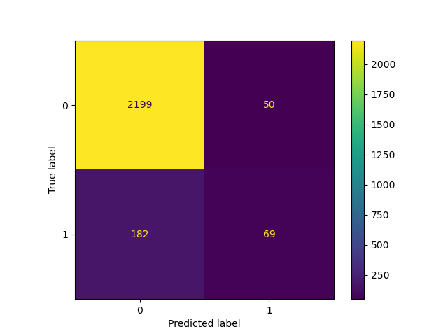
X, y = make_classification(n_samples=10_000, weights=[0.9, 0.1], random_state=0)
X_train, X_test, y_train, y_test = train_test_split(X, y, random_state=0)
classifier_05 = LogisticRegression(C=1e6, random_state=0).fit(X_train, y_train)
_ = ConfusionMatrixDisplay.from_estimator(classifier_05, X_test, y_test)
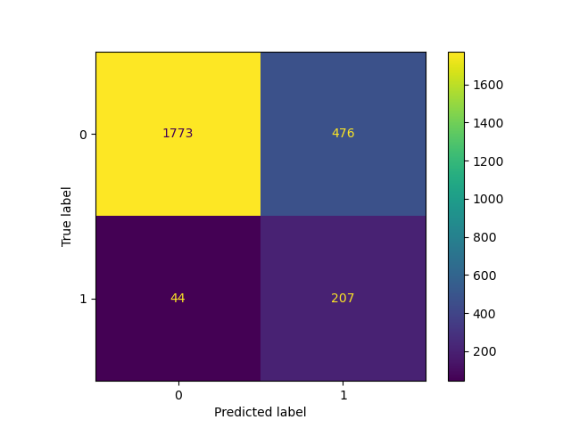
Lowering the threshold, i.e. allowing more samples to be classified as the positive class, increases the number of true positives at the cost of more false positives (as is well known from the concavity of the ROC curve).
from sklearn.model_selection import FixedThresholdClassifier

classifier_01 = FixedThresholdClassifier(classifier_05, threshold=0.1)
classifier_01.fit(X_train, y_train)
_ = ConfusionMatrixDisplay.from_estimator(classifier_01, X_test, y_test)
TunedThresholdClassifierCV: Tuning the decision threshold of a binary classifier#
The decision threshold of a binary classifier can be tuned to optimize a
given metric, using TunedThresholdClassifierCV.
It is particularly useful to find the best decision threshold when the model is meant to be deployed in a specific application context where we can assign different gains or costs for true positives, true negatives, false positives, and false negatives.
Let’s illustrate this by considering an arbitrary case where:
each true positive gains 1 unit of profit, e.g. euro, year of life in good health, etc.;
true negatives gain or cost nothing;
each false negative costs 2;
each false positive costs 0.1.
Our metric quantifies the average profit per sample, which is defined by the following Python function:
from sklearn.metrics import confusion_matrix


def custom_score(y_observed, y_pred):
    tn, fp, fn, tp = confusion_matrix(y_observed, y_pred, normalize="all").ravel()
    return tp - 2 * fn - 0.1 * fp


print("Untuned decision threshold: 0.5")
print(f"Custom score: {custom_score(y_test, classifier_05.predict(X_test)):.2f}")
Untuned decision threshold: 0.5
Custom score: -0.12
It is interesting to observe that the average gain per prediction is negative which means that this decision system is making a loss on average.
Tuning the threshold to optimize this custom metric gives a smaller threshold that allows more samples to be classified as the positive class. As a result, the average gain per prediction improves.
from sklearn.metrics import make_scorer
from sklearn.model_selection import TunedThresholdClassifierCV

custom_scorer = make_scorer(
    custom_score, response_method="predict", greater_is_better=True
)
tuned_classifier = TunedThresholdClassifierCV(
    classifier_05, cv=5, scoring=custom_scorer
).fit(X, y)

print(f"Tuned decision threshold: {tuned_classifier.best_threshold_:.3f}")
print(f"Custom score: {custom_score(y_test, tuned_classifier.predict(X_test)):.2f}")
Tuned decision threshold: 0.071
Custom score: 0.04
We observe that tuning the decision threshold can turn a machine learning-based system that makes a loss on average into a beneficial one.
In practice, defining a meaningful application-specific metric might involve making those costs for bad predictions and gains for good predictions depend on auxiliary metadata specific to each individual data point such as the amount of a transaction in a fraud detection system.
To achieve this, TunedThresholdClassifierCV
leverages metadata routing support (Metadata Routing User
Guide) allowing to optimize complex business metrics as
detailed in Post-tuning the decision threshold for cost-sensitive
learning.
Performance improvements in PCA#
PCA has a new solver, "covariance_eigh", which is
up to an order of magnitude faster and more memory efficient than the other
solvers for datasets with many data points and few features.
from sklearn.datasets import make_low_rank_matrix
from sklearn.decomposition import PCA

X = make_low_rank_matrix(
    n_samples=10_000, n_features=100, tail_strength=0.1, random_state=0
)

pca = PCA(n_components=10, svd_solver="covariance_eigh").fit(X)
print(f"Explained variance: {pca.explained_variance_ratio_.sum():.2f}")
Explained variance: 0.88
The new solver also accepts sparse input data:
Explained variance: 0.13
The "full" solver has also been improved to use less memory and allows
faster transformation. The default svd_solver="auto" option takes
advantage of the new solver and is now able to select an appropriate solver
for sparse datasets.
Similarly to most other PCA solvers, the new "covariance_eigh" solver can leverage
GPU computation if the input data is passed as a PyTorch or CuPy array by
enabling the experimental support for Array API.
ColumnTransformer is subscriptable#
The transformers of a ColumnTransformer can now be directly
accessed using indexing by name.
import numpy as np

from sklearn.compose import ColumnTransformer
from sklearn.preprocessing import OneHotEncoder, StandardScaler

X = np.array([[0, 1, 2], [3, 4, 5]])
column_transformer = ColumnTransformer(
    [("std_scaler", StandardScaler(), [0]), ("one_hot", OneHotEncoder(), [1, 2])]
)

column_transformer.fit(X)

print(column_transformer["std_scaler"])
print(column_transformer["one_hot"])
StandardScaler()
OneHotEncoder()
Custom imputation strategies for the SimpleImputer#
SimpleImputer now supports custom strategies for imputation,
using a callable that computes a scalar value from the non missing values of
a column vector.
from sklearn.impute import SimpleImputer

X = np.array(
    [
        [-1.1, 1.1, 1.1],
        [3.9, -1.2, np.nan],
        [np.nan, 1.3, np.nan],
        [-0.1, -1.4, -1.4],
        [-4.9, 1.5, -1.5],
        [np.nan, 1.6, 1.6],
    ]
)


def smallest_abs(arr):
    """Return the smallest absolute value of a 1D array."""
    return np.min(np.abs(arr))


imputer = SimpleImputer(strategy=smallest_abs)

imputer.fit_transform(X)
array([[-1.1,  1.1,  1.1],
       [ 3.9, -1.2,  1.1],
       [ 0.1,  1.3,  1.1],
       [-0.1, -1.4, -1.4],
       [-4.9,  1.5, -1.5],
       [ 0.1,  1.6,  1.6]])
Pairwise distances with non-numeric arrays#
pairwise_distances can now compute distances between
non-numeric arrays using a callable metric.
from sklearn.metrics import pairwise_distances

X = ["cat", "dog"]
Y = ["cat", "fox"]


def levenshtein_distance(x, y):
    """Return the Levenshtein distance between two strings."""
    if x == "" or y == "":
        return max(len(x), len(y))
    if x[0] == y[0]:
        return levenshtein_distance(x[1:], y[1:])
    return 1 + min(
        levenshtein_distance(x[1:], y),
        levenshtein_distance(x, y[1:]),
        levenshtein_distance(x[1:], y[1:]),
    )


pairwise_distances(X, Y, metric=levenshtein_distance)
array([[0., 3.],
       [3., 2.]])
Total running time of the script: (0 minutes 0.892 seconds)
Related examples
Post-hoc tuning the cut-off point of decision function
Post-tuning the decision threshold for cost-sensitive learning